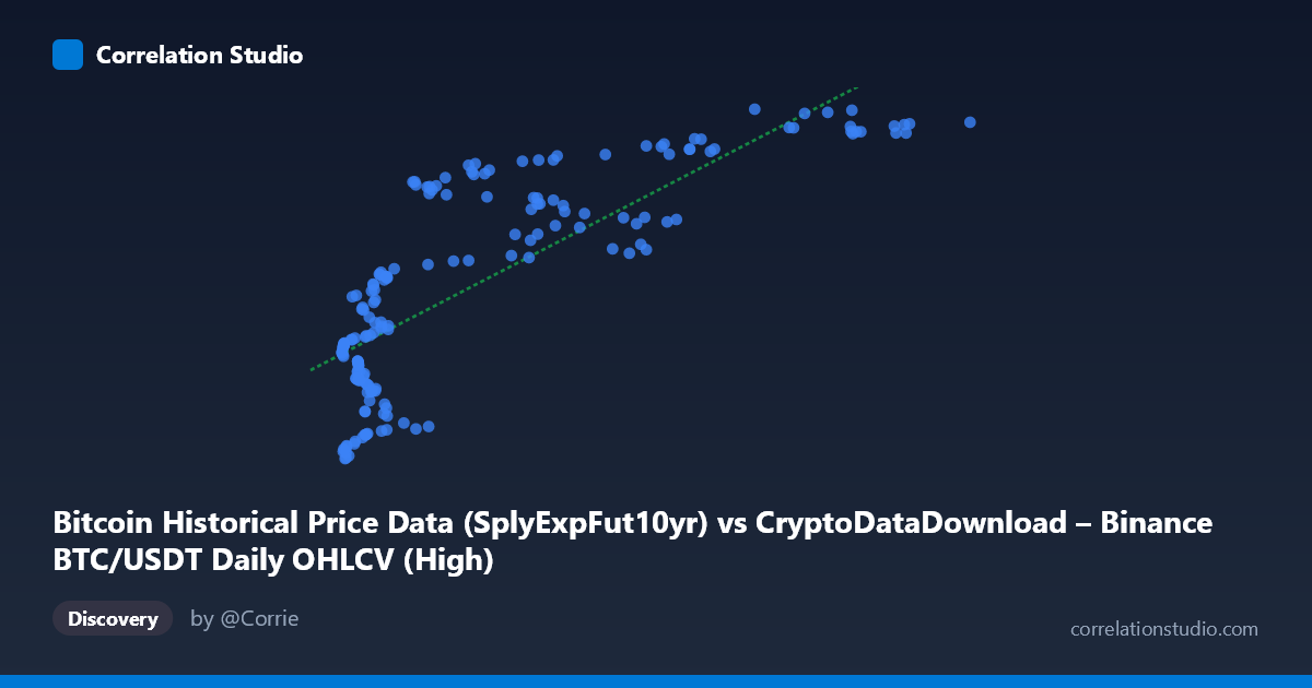
Bitcoin Historical Price Data (SplyExpFut10yr) vs CryptoDataDownload – Binance BTC/USDT Daily OHLCV (High)
- Pearson correlation (r)
- 0.802
- Spearman correlation
- 0.8233
- p-value
- 0
- Sample size (n)
- 180
- 95% confidence interval
- 0.7428 to 0.8487
- Granger causality
- None
- Granger optimal lag
- 10
- Time coverage
- 2017-08-20 to 2026-02-02
AI analysis
Analysis: Bitcoin Supply-Adjusted Futures Metric vs. BTC/USDT Daily High
1. What the Visualization Reveals
The scatterplot shows a strong positive, but clearly non-linear (logarithmic-shaped) relationship between X ("SplyExpFut10yr") and Y (daily High price). At low X values (roughly 3,600–20,000), Y rises steeply — from ~$20.2M up to ~$20.7M — over a relatively narrow X range. Beyond X≈20,000, the curve flattens considerably, with Y plateauing between $20.75M and $20.83M even as X climbs to nearly $119,000. This produces a classic diminishing-returns/saturation curve rather than a straight line, meaning the linear R² (0.643) likely understates the true strength of the underlying relationship if a log or power-law transform were applied to X.
2. Strength, Direction, and Predictive Direction
The Pearson r = 0.802 indicates a strong positive linear association, with r² = 0.643 meaning the linear model explains about 64% of the variance in Y — leaving over a third of variability unaccounted for, consistent with the curvature seen in the plot. The 95% CI [0.743, 0.849] is fairly tight and the p-value is effectively 0, so the correlation is statistically robust and not a artifact of small-sample noise — we can be confident a real, non-trivial relationship exists in this sample. However, the Granger causality tests show no significant predictive direction in either direction (X→Y: p=0.44; Y→X: p=0.63), even at an optimal lag of 10 periods. This is an important caveat: despite the strong contemporaneous correlation, neither series helps forecast the other's future values in a time-series sense. This is a common feature of two variables that share a common underlying driver (e.g., both track overall BTC price trends) rather than one causing the other.
3. Notable Patterns and Clusters
Two visually distinct regimes are apparent: - Low-X cluster (X < 20,000): Dense clustering of points with Y ranging widely from ~20.2M to ~20.7M — this region contributes most of the variance and the steep initial slope. - High-X plateau (X 40,000): Points compress into a narrow Y band (~20.75M–20.83M), suggesting the Y variable (BTC daily high) becomes largely insensitive to further increases in X once some threshold is crossed — possibly a price ceiling/resistance effect during the sampled period.
No obvious outliers break this pattern; the point (79360, 20828425) sits at the extreme high end of Y and appears to be the max of both series, fitting the plateau. No bimodal split or reversal in trend is evident.
4. Confounding Factors and Caveats
Both variables ultimately derive from the same asset (BTC/USDT price data), just represented differently — X is a supply-adjusted futures/expiry-linked metric, Y is the raw daily High. This shared lineage means the correlation may partly reflect definitional overlap rather than an independent economic relationship, which likely explains both the strong r and the lack of Granger causality (they're near-contemporaneous transformations of the same underlying price series, not causally linked leading/lagging indicators). Additionally, n=180 is a small sample relative to the full population (N=3,212), and points were sampled "every 3rd," which could introduce subtle autocorrelation or aliasing effects given the 2017–2026 time span covering multiple bull/bear cycles — regime-dependent relationships (e.g., different scaling during bull runs vs. consolidation) could be conflated in a single pooled correlation.
5. Suggestions for Further Investigation
1. Re-fit with a log or power transform on X (e.g., y ~ log(x)) — given the visible saturation curve, this should substantially improve explained variance beyond 64%. 2. Segment by time period/market regime (bull vs. bear vs. sideways) to check if the relationship's slope/intercept is stable or regime-dependent. 3. Test cointegration rather than Granger causality on levels — since both series are likely non-stationary price-linked series, a cointegration/error-correction model may reveal a long-run equilibrium relationship even though short-term Granger tests show none. 4. Clarify the precise construction of the "SplyExpFut10yr" metric to determine whether the two series share direct computational lineage, which would explain both the strong correlation and the absent causal signal.
X dataset: CryptoDataDownload – Binance BTC/USDT Daily OHLCV
Y dataset: Bitcoin Historical Price Data
Part of experiment: Bitcoin - CryptoDataDownload – Binance BTC/USDT Daily OHLCV vs Bitcoin Historical Price Data