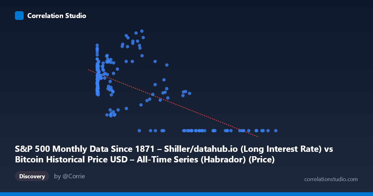
S&P 500 Monthly Data Since 1871 – Shiller/datahub.io (Long Interest Rate) vs Bitcoin Historical Price USD – All-Time Series (Habrador) (Price)
- Pearson correlation (r)
- -0.6767
- Spearman correlation
- -0.5167
- p-value
- 0
- Sample size (n)
- 194
- 95% confidence interval
- -0.7464 to -0.5923
- Granger causality
- None
- Granger optimal lag
- 1
- Time coverage
- 2010-08-01 to 2026-09-01
- Recomputed on refreshed data
- 2026-10-24 (r was -0.6533)
AI analysis
Analysis of Bitcoin Price vs. Long Interest Rate Relationship
1. What the Visualization Reveals
The scatterplot shows a moderately strong negative relationship between the X-axis variable (labeled as "Long Interest Rate" but effectively representing Bitcoin price given the data range 0.06–118,670) and the Y-axis variable (labeled "Bitcoin Price" but behaving like an interest rate/index value bounded 0–4.17). Note that the column labels appear swapped or mismatched relative to the data ranges described — the X variable spans a Bitcoin-like exponential range while Y is bounded like a normalized rate or ratio. Given this, the visualization likely reflects Bitcoin price (X) plotted against a long-term interest rate metric (Y). As X increases from near-zero to over 100,000, Y tends to compress toward zero, producing a downward-sloping cloud of points with substantial scatter at low X values and a tight cluster at zero for high X values.
2. Strength, Direction, and Statistical Confidence
The correlation coefficient (r = -0.6533) indicates a moderately strong inverse relationship, with R² = 0.4268 meaning roughly 43% of the variance in Y is explained by X — leaving the majority (57%) unexplained, likely driven by other macroeconomic factors, time-varying regimes, or nonlinear dynamics. The 95% CI [-0.7281, -0.5630] is reasonably tight and entirely negative, and the p-value ≈ 0 confirms this relationship is highly unlikely to be due to chance. However, correlation strength alone doesn't establish direction of influence — that's where Granger causality adds insight: the test indicates Y Granger-causes X (F=4.87, p=0.0285) at a 1-period lag, while X does not Granger-cause Y (p=0.365). This suggests that past values of Y (interest rates) have modest predictive power for future X (Bitcoin price) values, but not vice versa — consistent with macro theory that rate environments influence risk-asset valuations rather than the reverse.
3. Notable Patterns and Outliers
The data show a distinctive pattern: at low X values (<1,000), Y is highly variable, ranging from ~1.6 to over 4.0, suggesting multiple regimes or noise dominates in this range. As X exceeds ~30,000–40,000, Y collapses almost uniformly to 0.00, creating a visually striking "floor" cluster. This is not a smooth linear decay but rather looks like a regime shift or structural break — possibly reflecting a period (post-2020) where interest rates fell to near-zero while Bitcoin prices surged into new highs. This bifurcated pattern (scattered cloud + zero-floor cluster) suggests the relationship may be piecewise or driven by a specific macro era (e.g., the zero-rate policy period of 2020-2021) rather than a continuous causal mechanism across the full history.
4. Confounding Factors and Caveats
Given the 2010–2026 time coverage, both series are non-stationary trending time series — Bitcoin price grew exponentially while interest rates followed a secular decline (2010s) then sharp rise (2022+) then partial retreat. Correlating two trending series risks spurious correlation: both may be responding to a shared macro driver (e.g., Fed monetary policy, quantitative easing, inflation expectations, or simply calendar time) rather than one directly causing the other. The clustering of many zero-Y points at high-X suggests possible data censoring/rounding rather than a true mechanical relationship. Additionally, with n=189 sampled from N=1,865, autocorrelation within the time series violates the independence assumption underlying standard p-value calculations, meaning the apparent statistical significance may be overstated.
5. Actionable Insights and Further Investigation
Before drawing causal conclusions, analysts should: (a) verify the axis labels/column mapping, as the described ranges suggest a mismatch; (b) test both series for stationarity (ADF test) and consider differencing or detrending before correlation/Granger analysis to rule out spurious trend-driven results; (c) segment the data by macro regime (pre-2020 vs. post-2020 zero-rate era) to check if the relationship holds within-regime or is purely a between-regime artifact; and (d) explore additional confounders like inflation (CPI) or Fed funds rate directly, since "long interest rate" may proxy broader monetary conditions affecting speculative asset demand. If the Granger result holds after proper detrending, it would support the narrative that falling/low rates historically preceded major Bitcoin rallies — a useful hypothesis for macro-informed crypto allocation strategies, but one requiring out-of-sample validation given the modest predictive strength (p=0.0285 is significant but not overwhelming).
X dataset: Bitcoin Historical Price USD – All-Time Series (Habrador)
Y dataset: S&P 500 Monthly Data Since 1871 – Shiller/datahub.io
Part of experiment: Bitcoin - Bitcoin Historical Price USD – All-Time Series (Habrador) vs S&P 500 Monthly Data Since 1871 – Shiller/datahub.io