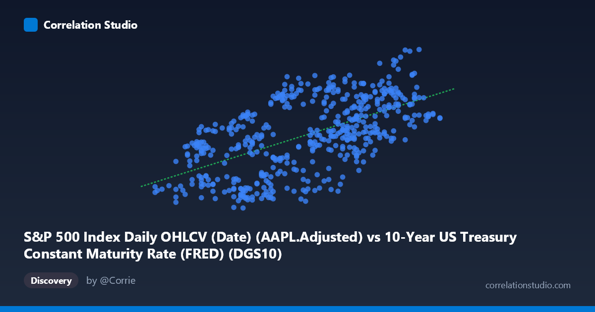
S&P 500 Index Daily OHLCV (Date) (AAPL.Adjusted) vs 10-Year US Treasury Constant Maturity Rate (FRED) (DGS10)
- Pearson correlation (r)
- 0.5912
- Spearman correlation
- 0.5923
- p-value
- 0
- Sample size (n)
- 502
- 95% confidence interval
- 0.5312 to 0.6453
- Granger causality
- X → Y
- Granger optimal lag
- 1
AI analysis
Analysis: S&P 500 (AAPL Adjusted) vs. 10-Year US Treasury Yield
1. Overall Relationship The scatterplot reveals a moderate positive relationship between the S&P 500 Apple adjusted price (X-axis) and the 10-year US Treasury constant maturity rate (Y-axis) over the period February 2015 to February 2017. As the equity price variable increases, Treasury yields tend to rise correspondingly, with the linear regression equation y = 21.21x + 67.54 capturing this upward trend. The data cloud is oriented positively but exhibits considerable vertical spread at nearly every level of X, indicating that the relationship, while real, is far from deterministic and is subject to substantial noise and other influences.
2. Correlation Strength and Statistical Significance The Pearson correlation of r = 0.591 indicates a moderate positive association. However, the r² value of 0.35 is the more telling statistic: only 35% of the variance in Treasury yields is explained by the S&P 500 price variable, leaving 65% attributable to other factors entirely. The 95% confidence interval of [0.531, 0.645] is reasonably tight and does not approach zero, and the p-value is effectively zero given n = 502, confirming this is not a chance finding. Critically, the Granger causality test supports a unidirectional predictive relationship: X Granger-causes Y (F = 6.02, p = 0.015) at a one-period lag, while the reverse direction fails to reach significance (F = 2.67, p = 0.103). This suggests that movements in the S&P 500/AAPL price series have some temporal predictive power over subsequent Treasury yield movements, though causation in the economic sense still cannot be fully established from this alone.
3. Notable Patterns, Clusters, and Outliers The data points cluster most densely in the X range of approximately 1.7–2.3 and Y range of 100–120, consistent with the reported means. There is a visible upper-right cluster of high-yield, high-price observations (X 2.3, Y 120), which appears to correspond to the post-2016 reflation trade when both equities and yields rose simultaneously — a "risk-on" regime. Conversely, a lower-left cluster near X ≈ 1.5–1.7 and Y ≈ 90–100 likely reflects early-2016 market stress. Several potential outliers are evident — notably points near (2.45, 135.35) and (2.43, 133.29) — representing episodes of unusually high yields relative to the fitted trend. Scatter is notably heteroscedastic, widening at higher X values, which suggests the relationship is less stable in bull market conditions.
4. Confounding Factors and Caveats Several important caveats apply. First, the axis labels appear to be swapped in the dataset metadata — AAPL adjusted prices are labeled as coming from the FRED Treasury dataset and vice versa, which warrants data provenance verification before drawing firm conclusions. Second, both variables are non-stationary time series that trended together during 2016's "Trump trade" reflation period, raising the possibility that the correlation is at least partly spurious co-trending rather than a structural relationship. Third, macroeconomic drivers — Federal Reserve policy shifts, inflation expectations, and risk sentiment — likely influence both variables simultaneously, acting as common confounders. Finally, using a single stock (AAPL adjusted) as a proxy for broad equity market conditions introduces idiosyncratic noise.
5. Actionable Insights and Further Investigation Given the Granger causality finding, practitioners could explore whether the one-period lag signal from equity prices to yields is exploitable in a tactical asset allocation or fixed income positioning framework, though the 35% explained variance ceiling suggests limited standalone utility. Further investigation should include: (a) first-differencing or detrending both series to test whether the correlation persists after removing common trends; (b) regime analysis to determine whether the correlation strengthens during risk-on vs. risk-off periods; (c) extending the analysis beyond the two-year window to test stability across multiple rate cycles; and (d) replacing AAPL adjusted prices with a broad index (SPX) to reduce idiosyncratic equity noise and improve the interpretability of the macro relationship being studied.
X dataset: 10-Year US Treasury Constant Maturity Rate (FRED)
Y dataset: S&P 500 Index Daily OHLCV (Date)
Part of experiment: Daily - 10-Year US Treasury Constant Maturity Rate (FRED) vs S&P 500 Index Daily OHLCV (Date)