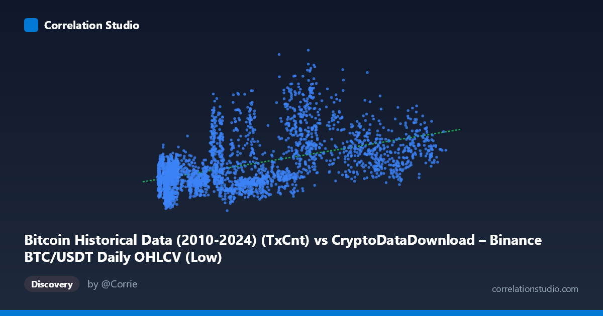
Bitcoin Historical Data (2010-2024) (TxCnt) vs CryptoDataDownload – Binance BTC/USDT Daily OHLCV (Low)
- Pearson correlation (r)
- 0.5052
- Spearman correlation
- 0.507
- p-value
- 0
- Sample size (n)
- 3191
- 95% confidence interval
- 0.4789 to 0.5306
- Granger causality
- None
- Granger optimal lag
- 10
- Time coverage
- 2017-08-17 to 2026-05-20
AI analysis
Analysis: Bitcoin Transaction Count vs. Price (Low)
1. What the Visualization Reveals
The scatterplot depicts the relationship between Bitcoin's daily transaction count (X-axis) and its daily low price (Y-axis) on Binance BTC/USDT, spanning nearly nine years (2017–2026). The data shows a clear positive but noisy relationship — as transaction counts increase, price lows tend to rise as well, but the spread around this trend is substantial. This is not a tight linear relationship; rather, it appears as a diffuse cloud with a discernible upward slope, suggesting transaction activity and price are related but far from deterministically linked.
2. Strength and Direction of the Correlation
The correlation coefficient (r = 0.505) indicates a moderate positive relationship. However, R² = 0.255 tells the more important story: only about 25.5% of the variance in price is explained by transaction count, leaving nearly three-quarters of price movement attributable to other factors. The 95% confidence interval [0.479, 0.531] is fairly tight given the large sample size (n=3,191), and the p-value of ~0 confirms this correlation is highly statistically significant — it is very unlikely to be due to chance. However, statistical significance here should not be conflated with practical strength; the relationship is real but weak-to-moderate in explanatory power.
Critically, the Granger causality tests show no significant predictive direction in either direction (X→Y: p=0.592; Y→X: p=0.889). This means neither transaction count nor price reliably "leads" the other in a time-series forecasting sense, even at an optimal lag of 10 periods. This is an important caveat: despite the contemporaneous correlation, transaction counts do not appear useful for predicting future price movements (or vice versa) based on this test.
3. Notable Patterns and Features
Several features stand out in the sample data: - Heteroscedasticity: Variance in Y appears to increase with X — at low transaction counts (~5,000-10,000), prices cluster in a tighter low range, while at higher transaction counts (~80,000-110,000), price spread widens considerably (e.g., points near x≈80,000 range from y≈412,000 to y≈531,000). - Non-linear suggestion: Some low-X, high-Y outliers exist (e.g., x=3,740, y=336,764 and x=9,080, y=378,081), suggesting price can be elevated even during lower on-chain activity — possibly reflecting speculative/derivative-driven price action decoupled from network usage. - Clustering: A dense cluster appears in the low-X (5,000–30,000) range, consistent with earlier years in the dataset when transaction counts were lower, while higher-X points likely correspond to later periods with network growth.
4. Potential Confounders and Caveats
Several confounding factors likely affect this relationship: - Time trend confounding: Both transaction count and price likely trended upward over the 2017-2026 period due to Bitcoin's overall adoption growth, market maturation, and halving cycles — creating a spurious correlation driven by shared temporal trends rather than direct causation. - Market regime shifts: Bull/bear cycles, macroeconomic conditions (rate changes, ETF approvals, regulatory news) likely drive price independent of on-chain transaction volume. - Mismatched units/scales: Transaction count reflects network usage, while "Low" price reflects market valuation — these may respond to different dynamics (e.g., speculation vs. utility). - Data source mismatch: X comes from one CDD dataset labeled with "TxCnt" while the column header suggests OHLCV origin — check for possible data alignment/merge errors between datasets.
5. Actionable Insights and Further Investigation
1. Detrend the data: Since both series likely have strong secular trends, consider using log returns or differenced/detrended series to test if the correlation holds after removing the time trend — this will clarify if the relationship is genuine or an artifact of co-trending. 2. Segment by market regime: Split data into bull/bear periods or by year to see if the r² is stable or driven by specific eras (e.g., 2020-2021 bull run). 3. Explore non-linear models: Given the heteroscedastic fan-shaped pattern, consider log-transforming X and/or Y, or testing polynomial/quantile regression to capture non-constant variance. 4. Reconsider causality assumptions: Given the lack of Granger causality, avoid using transaction count as a leading indicator for price forecasting; instead, treat both as jointly driven by external market factors. 5. Investigate outliers: Points with low transaction count but high price (or vice versa) merit deeper investigation — potentially tied to specific news events, exchange outages, or data quality issues.
X dataset: CryptoDataDownload – Binance BTC/USDT Daily OHLCV
Y dataset: Bitcoin Historical Data (2010-2024)
Part of experiment: Bitcoin - CryptoDataDownload – Binance BTC/USDT Daily OHLCV vs Bitcoin Historical Data (2010-2024)