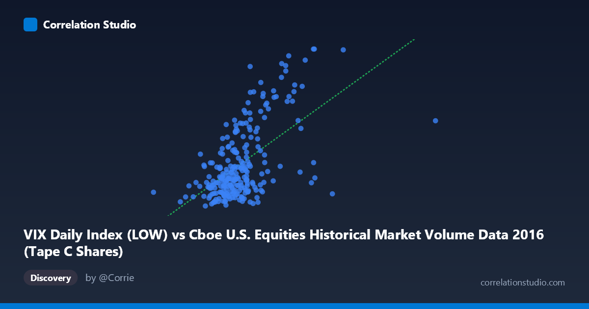
VIX Daily Index (LOW) vs Cboe U.S. Equities Historical Market Volume Data 2016 (Tape C Shares)
- Pearson correlation (r)
- 0.5723
- Spearman correlation
- 0.5065
- p-value
- 0
- Sample size (n)
- 252
- 95% confidence interval
- 0.4829 to 0.6499
- Granger causality
- None
- Granger optimal lag
- 1
AI analysis
Scatterplot Analysis: VIX Tape C Shares vs. VIX Daily Index (LOW)
Relationship Overview
The scatterplot reveals a moderate positive relationship between the VIX Daily Index (LOW) values on the X-axis and Tape C Shares volume on the Y-axis across 252 trading days in 2016. As the VIX low readings increase, Tape C share volume tends to rise correspondingly, which aligns intuitively with market behavior: when volatility expectations are elevated even at their daily lows, traders tend to be more active, driving higher equity volume. The linear regression equation (y = 7.69e-08x + 4.94) confirms this positive slope, though the relatively small coefficient reflects the vast scale difference between the two variables.
Correlation Strength and Statistical Significance
The correlation of r = 0.5723 indicates a moderate positive association, with r² = 0.3275 meaning that roughly 32.8% of the variance in Tape C Shares is explained by the VIX Low index — leaving approximately 67% attributable to other factors. The 95% confidence interval of [0.4829, 0.6499] is reasonably tight and does not cross zero, and the p-value of effectively 0 confirms this relationship is highly statistically significant across the N = 3,622 population. However, the Granger causality tests complicate the narrative considerably: neither direction (X→Y: F = 0.1133, p = 0.737; Y→X: F = 0.0557, p = 0.814) achieves significance at any conventional threshold, meaning neither variable reliably predicts the other temporally at a one-period lag. Correlation exists contemporaneously, but neither series leads the other in a forecasting sense.
Notable Patterns, Clusters, and Outliers
Several structural features stand out in the data. The bulk of observations cluster tightly in the X range of roughly 100–160 million (VIX Low) and Y range of 11–18 (Tape C Shares), forming a dense core. However, there are notable outliers pulling the regression line: one point near (175M, 25.0) and another near (166M, 21.9) represent high-volatility, high-volume days that likely correspond to specific market stress events in 2016 (e.g., Brexit in late June or the U.S. election in November). There also appear to be a handful of points with very high X values (above 200M, extending toward 315M) that do not necessarily carry proportionally high Y values, suggesting the linear relationship may weaken or break down at extreme volume levels. This hints at a possible non-linear or heteroscedastic structure where variance in Y increases with X.
Confounding Factors and Caveats
Several important caveats apply. First, the axis assignment appears analytically inverted — VIX data (a volatility index) is plotted on X while market volume (Tape C Shares) is on Y, yet intuitively volatility might better serve as the dependent variable or the axes could reflect a data-joining artifact. Second, Tape C Shares represent only a subset of total equity market volume (NYSE Arca-listed securities), so the relationship may not generalize to the broader market. Third, 2016 was an unusually event-dense year (Brexit, U.S. presidential election), which could artificially inflate the correlation through shared responses to common macro shocks rather than any direct mechanical link between these two variables. Finally, the lack of Granger causality at a one-period lag does not rule out relationships at longer lags or in transformed (e.g., log-differenced) form.
Actionable Insights and Further Investigation
Practitioners should avoid using this relationship for short-term directional trading signals, given the failed Granger causality tests — knowing yesterday's VIX Low does not improve predictions of today's Tape C volume, and vice versa. However, the contemporaneous correlation (r ≈ 0.57) suggests these variables may respond jointly to common underlying drivers worth isolating. Recommended next steps include: (1) testing Granger causality at longer lags (2–5 periods) to check for delayed transmission effects; (2) applying log transformations to both variables to address potential heteroscedasticity visible at high X values; (3) segmenting the data around known shock events (Brexit, election) to determine whether the correlation is event-driven or structural; and (4) incorporating additional variables such as the VIX High or VIX Close, total market volume, and bid-ask spreads to build a more complete multivariate model of what drives Tape C share activity.
X dataset: Cboe U.S. Equities Historical Market Volume Data 2016
Y dataset: VIX Daily Index
Part of experiment: Daily - Cboe U.S. Equities Historical Market Volume Data 2016 vs VIX Daily Index