World Bank CO2 Emissions by Country (DataBank) (Bunker fuels (Not in Total)) vs US Employment and Unemployment (nonagriculture_ratio)
- Pearson correlation (r)
- 0.9534
- Spearman correlation
- 0.9714
- p-value
- 0
- Sample size (n)
- 80
- 95% confidence interval
- 0.9281 to 0.9699
- Granger causality
- None
- Granger optimal lag
- 10
AI analysis
Scatterplot Analysis: Bunker Fuel CO₂ Emissions vs. US Non-Agricultural Employment Ratio
Relationship Overview
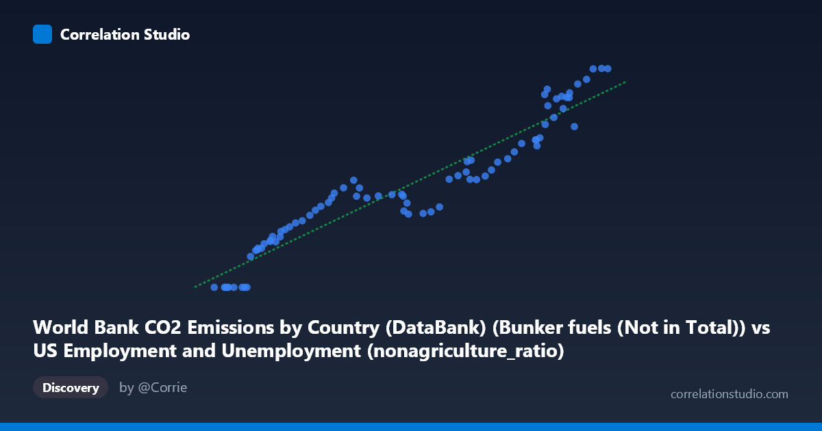
The scatterplot reveals a strong, positive, and largely linear relationship between global bunker fuel CO₂ emissions (X-axis) and the US non-agricultural employment ratio (Y-axis) across the period 1941–2020. As bunker fuel emissions increase, the non-agricultural employment ratio rises in near-lockstep, tracing a clear upward trajectory from the lower-left to the upper-right of the plot. The linear regression equation (y = 0.0119652x − 424.692) captures this trend well, and visually the data points cluster tightly around the regression line across most of the range, suggesting a remarkably consistent co-movement over eight decades of annual observations.
Correlation Strength and Statistical Interpretation
The Pearson correlation coefficient of r = 0.9534 indicates an exceptionally strong positive association, and the R² value of 0.9089 means that approximately 90.9% of the variance in the US non-agricultural employment ratio is statistically explained by variation in bunker fuel CO₂ emissions. The 95% confidence interval for r [0.9281, 0.9699] is narrow, confirming the estimate is stable and precise across the sample of n = 80 paired observations. The p-value of effectively zero rules out any plausible chance explanation. However, the Granger causality results complicate any causal narrative: neither direction (X→Y: F = 2.02, p = 0.051; Y→X: F = 1.72, p = 0.102) clears the conventional significance threshold, even at the optimal lag of 10 periods. This means that neither variable reliably predicts future values of the other in a temporal sense — the correlation, while visually and statistically compelling, does not establish predictive directionality.
Notable Patterns, Clusters, and Outliers
The most structurally distinctive feature is a cluster of zero-valued Y observations at the lower end of the X range (roughly X ∈ [41,250–51,000]), including multiple data points where the non-agricultural ratio is recorded as exactly 0.00. These likely reflect early wartime or immediate post-war years (early 1940s) where employment categorization or data availability differs from later periods, and they appear as a discrete floor rather than a smooth continuation of the linear trend. At the upper end (X 140,000), several points approach a visible ceiling near Y ≈ 1,590, suggesting possible saturation or a natural upper bound in the non-agricultural ratio. The mid-range (X ∈ [60,000–120,000]) shows the tightest adherence to linearity with minimal scatter, while variance appears slightly wider at the extremes.
Confounding Factors and Interpretive Caveats
This correlation almost certainly reflects shared secular trends rather than a direct structural relationship. Both variables are strongly time-driven: global economic growth over the 20th century simultaneously drove industrialization (increasing bunker fuel use in maritime and aviation transport) and expanded formal non-agricultural labor markets in the US. This is a textbook example of spurious correlation via a common latent driver — long-run economic development. The dataset mismatch also warrants caution: bunker fuel emissions are a global measure excluded from national totals, while the employment ratio is a US-specific metric, making any direct mechanism implausible. Furthermore, the zero-floor cluster in early years may reflect data encoding choices rather than true zero employment ratios, which would artificially inflate the linearity of the fit.
Actionable Insights and Further Investigation
Given the absence of Granger causality in either direction, further analysis should focus on detrending both series (e.g., using first differences or HP filtering) to isolate short-term co-movements from the shared long-run growth trend — if the correlation collapses after detrending, the relationship is almost entirely spurious. It would also be valuable to test whether a third variable, such as global GDP, world trade volume, or US industrial output, mediates or eliminates this correlation entirely when included in a multivariate model. The apparent saturation at the upper end of Y suggests investigating whether the non-agricultural ratio has structural limits, and whether post-2000 data (likely the upper-right cluster) follows a different regime than mid-century observations. Finally, the 10-period optimal lag in the Granger test is worth exploring further — borderline p-values at longer lags may hint at weak but real delayed feedback worth modeling with more flexible time-series approaches.
X dataset: US Employment and Unemployment
Y dataset: World Bank CO2 Emissions by Country (DataBank)
Part of experiment: Yearly - US Employment and Unemployment vs World Bank CO2 Emissions by Country (DataBank)