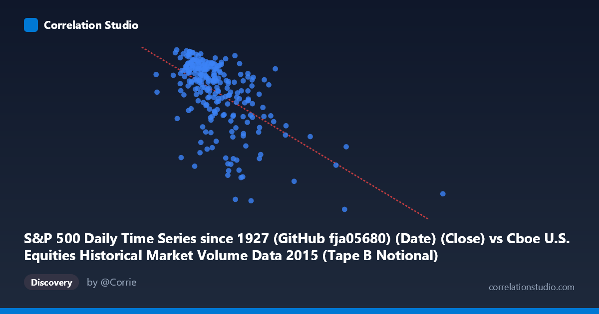
S&P 500 Daily Time Series since 1927 (GitHub fja05680) (Date) (Close) vs Cboe U.S. Equities Historical Market Volume Data 2015 (Tape B Notional)

Pearson correlation (r): -0.5707
Spearman correlation: -0.5618
p-value: 0
Sample size (n): 252
95% confidence interval: -0.6485 to -0.481
Granger causality: None
Granger optimal lag: 7

AI analysis

Analysis: S&P 500 Close Price vs. Cboe Tape B Notional Volume (2015)

1. Overall Relationship The scatterplot reveals a moderate negative relationship between the S&P 500 daily closing price and Cboe Tape B notional trading volume throughout 2015. As the S&P 500 close price increases, Tape B notional volume tends to decrease, and conversely, the largest volume spikes cluster around periods of lower index prices. The linear regression equation (y = -1.80×10⁻⁸x + 2159.32) captures this inverse trend, though the scatter is substantial, indicating considerable unexplained variability around the fitted line.

2. Correlation Strength, Direction, and Predictive Value The correlation of r = -0.5707 reflects a moderate negative association. Practically, this means higher S&P 500 closing prices tend to coincide with lower Tape B notional volumes — consistent with the well-known phenomenon that elevated market volatility and price stress drive trading activity. However, r² = 0.3257 tells a sobering story: only about 32.6% of the variance in Tape B notional volume is explained by the S&P 500 close price, leaving roughly 67% attributable to other factors. The 95% confidence interval of [-0.6485, -0.4810] is moderately tight and does not cross zero, and the p-value of effectively 0 confirms the correlation is highly statistically significant with N = 3,302. Despite statistical significance, the Granger causality results are notably absent in both directions — neither X→Y (F = 1.923, p = 0.067) nor Y→X (F = 0.868, p = 0.533) reaches significance at conventional thresholds. This means that while the two variables are contemporaneously correlated, neither reliably predicts the other in a temporal, lead-lag sense, which is an important practical limitation for any trading or forecasting application.

3. Notable Patterns, Clusters, and Outliers The sample points reveal a clear high-volume cluster at lower price levels (S&P 500 closes roughly in the 1867–1970 range), which aligns with the August–September 2015 market correction — a period of sharp drawdowns and elevated volatility that naturally drives notional volume higher. The bulk of observations concentrate between approximately 3.5–6.5 billion on the X-axis with S&P prices in the 2040–2130 range, forming a dense core cluster. Several notable outliers appear at extreme X values (e.g., ~12.5 billion and ~17.9 billion), with lower Y values, which may reflect end-of-year rebalancing or index reconstitution events. The relationship also appears somewhat heteroscedastic, with variance in Y increasing at lower X values, suggesting the negative correlation is partly driven by a handful of high-stress trading days rather than a uniform linear trend.

4. Confounding Factors and Caveats Several important caveats apply. First, market regime effects are likely driving much of this correlation — the 2015 August correction created simultaneous low prices and high volumes, making the two variables appear structurally linked when they may simply be joint responses to volatility. Tape B specifically covers NYSE American (AMEX) and regional exchange stocks, so this is not a whole-market volume measure, potentially introducing compositional biases. The date variable on the X-axis (encoded as Unix timestamps) is unusual — the correlation may partly reflect a time-series trend rather than a pure cross-sectional relationship between price and volume. Additionally, notional volume is price-sensitive by construction (shares × price), which could create mechanical correlations that don't reflect genuine behavioral relationships between S&P price levels and trading activity.

5. Actionable Insights and Further Investigation Given that Granger causality is absent, practitioners should not use S&P 500 close prices as a predictive signal for Tape B notional volume in a forecasting context. However, the contemporaneous correlation does suggest that volatility (VIX) or realized variance — rather than price levels — may be the underlying driver worth modeling directly. Further investigation should include: (1) regressing volume on VIX or intraday range to test whether volatility explains more variance than price level alone; (2) decomposing the time series to separate trend, seasonality, and shock effects before computing correlations; (3) isolating the August–September correction period to test whether the correlation holds outside stress periods; and (4) examining share volume vs. notional volume to disentangle the mechanical price-scaling effect from behavioral trading patterns.

X dataset: Cboe U.S. Equities Historical Market Volume Data 2015

Y dataset: S&P 500 Daily Time Series since 1927 (GitHub fja05680) (Date)

Part of experiment: Daily - Cboe U.S. Equities Historical Market Volume Data 2015 vs S&P 500 Daily Time Series since 1927 (GitHub fja05680) (Date)