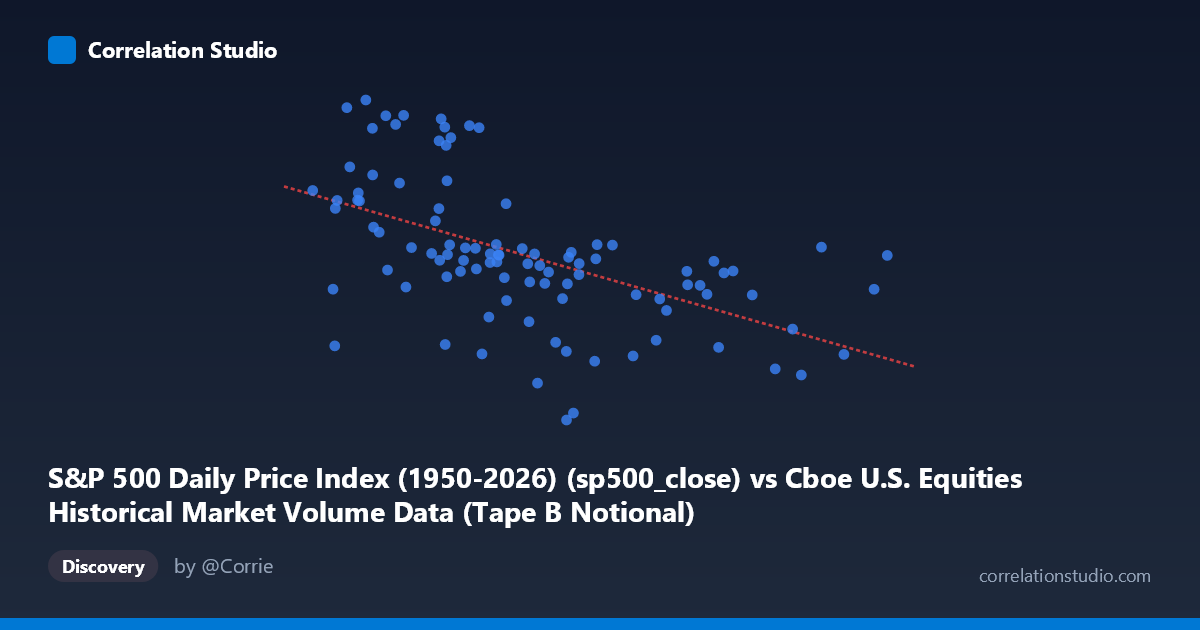
S&P 500 Daily Price Index (1950-2026) (sp500_close) vs Cboe U.S. Equities Historical Market Volume Data (Tape B Notional)
- Pearson correlation (r)
- -0.5397
- Spearman correlation
- -0.6197
- p-value
- 0
- Sample size (n)
- 98
- 95% confidence interval
- -0.6667 to -0.3822
- Granger causality
- None
- Granger optimal lag
- 10
AI analysis
Scatterplot Analysis: S&P 500 Price vs. Tape B Notional Trading Volume
Relationship Overview
The scatterplot reveals a moderate negative relationship between the S&P 500 daily closing price and Cboe Tape B notional trading volume, captured over the first five months of 2026 (January 2 through May 22). As the S&P 500 price index rises, Tape B notional volume tends to decline, and conversely, lower price levels are associated with elevated notional trading activity. The linear regression equation (y = −4.28×10⁻⁸x + 7,463.1) quantifies this: for every one-unit increase in the S&P 500 index, Tape B notional volume decreases by approximately 0.0428 units, anchored around a baseline of ~7,463. This inverse pattern suggests that market stress or price dislocation periods — typically coinciding with lower index levels — drive higher notional volume on mid-cap and regional exchange-listed securities (Tape B covers NYSE American, NYSE Arca, and regional exchanges).
Correlation Strength, Statistical Significance, and Causality
The Pearson correlation of r = −0.5397 indicates a moderate negative association, and the explained variance of r² = 0.2913 means that approximately 29.1% of the variance in Tape B notional volume is accounted for by the S&P 500 price level — a meaningful but far from complete explanation, leaving roughly 71% attributable to other factors. The result is highly statistically significant (p = 9.778×10⁻⁹), making it extremely unlikely this correlation arose by chance in the sample of n = 98 paired observations drawn from a population of N = 1,980. The 95% confidence interval for r [−0.667, −0.382] is comfortably negative throughout, reinforcing confidence in the direction of the relationship, though the relatively wide interval (~0.28 wide) signals meaningful uncertainty about the precise magnitude. Critically, Granger causality tests find no significant predictive direction in either direction (X→Y: F = 0.856, p = 0.578; Y→X: F = 1.037, p = 0.423), even at an optimal lag of 10 periods. This means that while the two variables co-move, neither reliably leads or predicts the other temporally — the correlation reflects contemporaneous co-movement, not a lagged causal mechanism exploitable for forecasting.
Notable Patterns, Clusters, and Outliers
Several structural features are visible in the data. There is a pronounced cluster of observations in the S&P 500 range of approximately 9.8–13.5 billion (x-axis), where Tape B notional volume spans a wide band from roughly 6,600 to 7,500 — indicating high within-cluster variance that the linear model cannot resolve. At the higher end of S&P 500 values (17–21 billion range), volume generally compresses toward the 6,500–6,900 range, with less dispersion, suggesting the inverse relationship tightens at elevated price levels. Several potential outliers are evident: the points near (13,233,916,266; 6,343.72) and (13,400,251,082; 6,368.85) show unusually low Tape B volume for their price level, falling well below the regression line, possibly reflecting low-volume trading days (holidays, shortened sessions) or data anomalies. Conversely, points such as (8,390,501,361; 7,501.24) and (9,302,436,398; 7,445.72) represent high-volume, low-price episodes consistent with market sell-off or volatility events. The scatter also hints at a possible non-linear (concave) structure — volume declines steeply as prices rise from low levels but may plateau at higher price levels — suggesting a simple linear fit may be suboptimal.
Confounding Factors and Interpretive Caveats
Several important caveats limit causal interpretation. Notional volume is price-dependent by construction: because notional value = shares × price, a declining S&P 500 (as a broad market proxy) mechanically reduces per-share prices across listed securities, which would reduce notional values even if share volume (count) remained constant. This creates a mathematical artifact in the correlation that may overstate the behavioral relationship. Additionally, the Tape B dataset label appears to be swapped with the S&P 500 dataset in the axis descriptions (the dataset names in the metadata are reversed), which warrants verification before drawing firm conclusions. The five-month time window (January–May 2026) captures a single market regime, potentially including specific macro events (Federal Reserve decisions, earnings seasons, geopolitical shocks) that could drive both variables simultaneously — a classic omitted variable / confounding scenario. The lack of Granger causality at up to 10 lags also suggests that any relationship may be driven by simultaneous external shocks (e.g., risk-off events) rather than a durable structural link.
Actionable Insights and Further Investigation
Practitioners and researchers should consider several follow-up steps. First, decompose notional volume into share count volume to isolate whether the observed inverse correlation is a mathematical artifact of price-dependent notional calculation or a genuine behavioral signal of increased trading activity during downturns. Second, test for non-linear specifications (e.g., logarithmic or quadratic regression) given the visual suggestion of a concave relationship; the current linear model's r² of 0.29 likely leaves systematic structure on the table. Third, extend the time series beyond five months to assess whether this inverse relationship holds across multiple market regimes (bull markets, prolonged bear markets, high-volatility regimes) — a single-year window is insufficient to establish a durable structural relationship. Fourth, incorporate volatility measures (VIX, realized variance) as control variables, since volatility simultaneously suppresses prices and amplifies trading activity, likely acting as a significant omitted confounder. Finally, verify dataset axis alignment given the apparent metadata label reversal, as correct variable assignment is foundational to any analytical conclusions drawn from this correlation.
X dataset: Cboe U.S. Equities Historical Market Volume Data
Y dataset: S&P 500 Daily Price Index (1950-2026)
Part of experiment: Daily - Cboe U.S. Equities Historical Market Volume Data vs S&P 500 Daily Price Index (1950-2026)