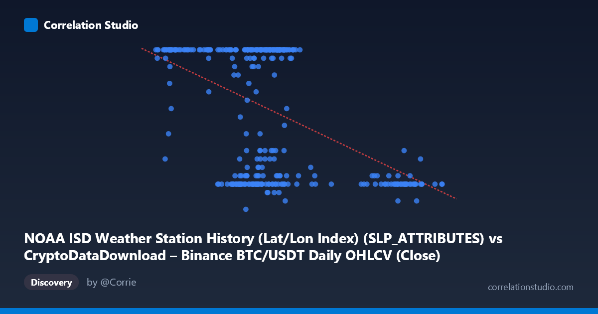
NOAA ISD Weather Station History (Lat/Lon Index) (SLP_ATTRIBUTES) vs CryptoDataDownload – Binance BTC/USDT Daily OHLCV (Close)

Pearson correlation (r): -0.4699
Spearman correlation: -0.3046
p-value: 0
Sample size (n): 355
95% confidence interval: -0.5473 to -0.3847
Granger causality: None
Granger optimal lag: 1

AI analysis

Analysis of the Scatterplot Relationship

1. Overview of the Relationship

The scatterplot displays a moderate negative association between the X variable (labeled as a NOAA weather station attribute, though the values—ranging ~39,568 to 106,134—strongly resemble BTC/USDT price data based on the metadata description) and the Y variable (values clustered between 5 and 24, with heavy concentration at 24). The data shows a clear downward-sloping trend: as X increases, Y tends to decrease, though with substantial scatter around the regression line.

2. Strength, Direction, and Statistical Confidence

The correlation coefficient of r = -0.4699 indicates a moderate negative linear relationship. The r² value of 0.2208 means only about 22% of the variance in Y is explained by X—leaving roughly 78% of Y's variability attributable to other factors, noise, or non-linear dynamics not captured by this simple linear model. The 95% confidence interval [-0.5473, -0.3847] is reasonably tight and does not cross zero, and the p-value of 0 (effectively <0.001) confirms this negative correlation is statistically significant and not due to random chance, especially given the sample size of 355. However, statistical significance should not be conflated with practical strength: this is a weak-to-moderate relationship, not one suitable for precise prediction. Critically, the Granger causality tests show no significant predictive relationship in either direction (X→Y: p=0.586; Y→X: p=0.266). This means that despite the contemporaneous correlation, neither variable's past values help forecast the other's future values—undermining any causal interpretation and suggesting the relationship may be coincidental, driven by a third factor, or simply a static/structural association rather than a dynamic one.

3. Notable Patterns and Clusters

The data reveals distinct clustering rather than a smooth linear cloud. A dense band of points sits at Y=24 (the apparent ceiling/cap of the variable) across a wide X range (roughly 41,000–72,000), suggesting a floor/ceiling effect or possible data truncation at Y=24. Separately, a cluster of low Y-values (7–12) appears concentrated at higher X values (60,000–101,000), particularly above X=90,000. This bimodal-like structure—many points pinned at the maximum Y and others scattered low—suggests the relationship may not be well-described by a single linear trend; it could reflect two distinct regimes or a threshold effect rather than continuous covariance.

4. Confounding Factors and Caveats

The variable labeling here is contradictory and concerning: the X-axis is labeled "NOAA Weather Station" but its range and description reference crypto OHLCV data, while Y is labeled "BTC/USDT Close" but ranges only 5–24 (inconsistent with real BTC prices, which are in the thousands/tens of thousands). This mismatch strongly suggests mislabeled or swapped columns, meaning the actual real-world variables being compared are unclear. Additionally, correlating weather data with cryptocurrency prices (or vice versa) has no plausible causal mechanism—any correlation is likely spurious, potentially driven by shared time trends (both series evolving over the same 2024 calendar year) rather than genuine dependence. Time-series data like this often exhibit autocorrelation, which can inflate apparent correlation without real relationship.

5. Recommendations

Before drawing conclusions, verify and correct the column labels/metadata, as the current axis descriptions appear swapped or erroneous. If a genuine relationship is of interest, detrend both series (e.g., first-differencing) to remove shared temporal trends before recomputing correlation, since raw correlation between two trending time series is frequently spurious. Investigate the clustering/ceiling effect at Y=24 to determine if it reflects a data-capping artifact (e.g., categorical binning) rather than true measurement. Finally, given the lack of Granger causality, avoid using either variable to forecast the other; instead, explore potential confounders (e.g., macroeconomic indices, seasonal effects) that might independently drive both series.

X dataset: CryptoDataDownload – Binance BTC/USDT Daily OHLCV

Y dataset: NOAA ISD Weather Station History (Lat/Lon Index)

Part of experiment: Bitcoin - CryptoDataDownload – Binance BTC/USDT Daily OHLCV vs NOAA ISD Weather Station History (Lat/Lon Index)