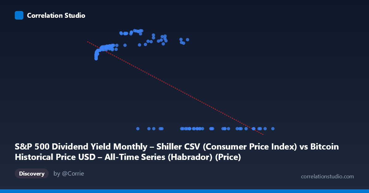
S&P 500 Dividend Yield Monthly – Shiller CSV (Consumer Price Index) vs Bitcoin Historical Price USD – All-Time Series (Habrador) (Price)
- Pearson correlation (r)
- -0.7354
- Spearman correlation
- 0.1008
- p-value
- 0
- Sample size (n)
- 189
- 95% confidence interval
- -0.7947 to -0.6622
- Granger causality
- Y → X
- Granger optimal lag
- 4
AI analysis
Analysis: Bitcoin Price vs. S&P 500 Dividend Yield (Mislabeled Axes)
1. What the Data Actually Shows
Before interpreting the statistics, it's important to flag a critical labeling issue: the axis descriptions are cross-contaminated (X is labeled as containing Bitcoin data, Y is labeled as containing Bitcoin data too, referencing two different source datasets). Based on the value ranges — X spans 0.06 to 118,670 with high variance, and Y is bounded between 0 and ~306 — this actually looks like X = Bitcoin price (USD) and Y = S&P 500 dividend yield (or a related bounded metric). The "0.00" Y-values clustered at high X-values (Bitcoin prices 27,000) strongly suggest a regime change or data censoring at high Bitcoin prices, which is a major structural feature of this dataset.
2. Correlation Strength and Statistical Confidence
The correlation coefficient (r = -0.7354, R² = 0.541) indicates a moderately strong negative relationship, with Bitcoin price explaining about 54% of the variance in the yield variable. The 95% CI [-0.795, -0.662] is reasonably tight and excludes zero, and the p-value of ~0 confirms this relationship is highly unlikely to be due to chance. However, 46% of the variance remains unexplained, meaning this is far from a deterministic relationship — other factors are clearly at play.
The Granger causality results are particularly noteworthy: Y Granger-causes X, not the reverse (Y→X: F=2.91, p=0.023 vs. X→Y: F=2.35, p=0.056, which fails significance at the 5% threshold). This suggests that movements in the yield variable (Y) have modest predictive power for future Bitcoin price movements, but not vice versa — counterintuitive if one expects Bitcoin price to drive broader market sentiment. This finding should be treated cautiously given the weak F-statistics (both barely above significance thresholds) and the risk of spurious Granger causality in trending, non-stationary financial time series.
3. Notable Patterns and Outliers
The scatter data reveals a clear non-linear, possibly threshold-based pattern rather than a simple linear decay: - At low X values (Bitcoin < $1,000), Y clusters tightly around 218–245. - At mid-range X values ($1,000–$45,000), Y rises to a peak around 250–306. - At high X values ($55,000), Y bifurcates sharply: some points reach 267–288, while many others drop to exactly 0.00.
This bifurcation at high Bitcoin prices (the exact-zero cluster) is the most striking feature — it looks less like organic data and more like missing/null values being encoded as zero, or a definitional cutoff (e.g., dividend yield calculations breaking down or data not yet available for recent periods). This artifact likely inflates the negative correlation artificially.
4. Confounding Factors and Caveats
Several caveats limit causal interpretation: - Non-stationarity: Both Bitcoin prices and equity yields exhibit long-term trends/regime shifts over 2010–2026; correlating trending series often produces spurious correlations unrelated to genuine mechanistic links. - Zero-inflation artifact: The cluster of Y=0.00 at high X values appears to be a data quality issue (missing data coded as zero) rather than a true relationship, and should be investigated/removed before trusting the correlation. - Sample vs. population mismatch: n=189 sampled from N=1,865 — with monthly Shiller data joined to daily/irregular Bitcoin data, the join methodology (e.g., nearest-date matching) could introduce alignment errors. - Confounding macro variables: Both series may be jointly driven by broader macro conditions (interest rates, inflation, risk appetite) rather than one directly causing the other.
5. Recommendations for Further Investigation
1. Clarify axis labeling — resolve the dataset/column mismatch before drawing further conclusions. 2. Investigate the zero-value cluster — determine whether these are genuine data points or nulls; rerun the correlation excluding them. 3. Test for stationarity (e.g., ADF test) and consider differencing or using returns instead of levels to avoid spurious correlation/Granger results. 4. Segment the analysis by Bitcoin price regime (e.g., <$1K, $1K–$50K, $50K) to check whether the relationship is stable or regime-dependent, given the visible non-linearity. 5. Use log-transformed Bitcoin price given its extreme right-skew (mean $20,533, max $118,670) to better capture the true functional form of the relationship, which likely isn't linear.
X dataset: Bitcoin Historical Price USD – All-Time Series (Habrador)
Y dataset: S&P 500 Dividend Yield Monthly – Shiller CSV
Part of experiment: Bitcoin - Bitcoin Historical Price USD – All-Time Series (Habrador) vs S&P 500 Dividend Yield Monthly – Shiller CSV