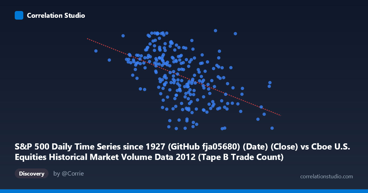
S&P 500 Daily Time Series since 1927 (GitHub fja05680) (Date) (Close) vs Cboe U.S. Equities Historical Market Volume Data 2012 (Tape B Trade Count)

Pearson correlation (r): -0.4925
Spearman correlation: -0.533
p-value: 0
Sample size (n): 250
95% confidence interval: -0.5811 to -0.3925
Granger causality: X → Y
Granger optimal lag: 1

AI analysis

Analysis: S&P 500 Closing Price vs. Cboe Tape B Trade Count (2012)

Relationship Overview The scatterplot reveals a negative relationship between the S&P 500 daily closing price (X-axis) and Cboe Tape B trade count (Y-axis) across 2012. As the S&P 500 index level rises throughout the year, the number of trades recorded on Tape B venues tends to decline. This inverse pattern is visually apparent in the downward slope of the regression line (y = −0.000574x + 1,480.16), and aligns with a broader market narrative: as equity prices recovered and trended upward in 2012, trading activity — particularly on Tape B venues covering NYSE Arca-listed securities — gradually contracted, consistent with declining volatility and reduced speculative churn in a calmer bull market environment.

Correlation Strength and Statistical Significance The Pearson correlation of r = −0.4925 indicates a moderate negative association. However, the coefficient of determination (R² = 0.2426) is the more sobering metric: only ~24.3% of the variance in Tape B trade count is explained by the S&P 500 price level, meaning roughly three-quarters of day-to-day variation in trade count is driven by factors outside this simple linear model. The 95% confidence interval for r [−0.5811, −0.3925] is meaningfully narrow given n = 250, and the p-value of effectively zero confirms the relationship is highly unlikely to be a sampling artifact — this is a statistically robust, if modest, association. Critically, Granger causality testing provides directional evidence: X Granger-causes Y (F = 4.95, p = 0.027) at a one-period lag, while the reverse direction fails to achieve significance (F = 0.67, p = 0.412). This suggests that S&P 500 price movements have modest predictive utility for next-period Tape B trade counts, but not vice versa — trade volume does not appear to lead price at this temporal resolution.

Patterns, Clusters, and Outliers The sample points reveal considerable vertical scatter at any given price level, reinforcing the modest R². Several notable features stand out. At lower index values (~105,000–165,000 range, representing earlier 2012 when prices were lower), trade counts span a wide band from roughly 1,277 to 1,447 — suggesting high day-to-day variability during periods of market uncertainty. At higher price levels (200,000–295,000), trade counts compress somewhat toward the 1,310–1,395 range, consistent with lower volatility regimes generating less frequent trading. One notable outlier appears near (222,649; 1,465.77) — a high price level paired with an unusually elevated trade count — and another cluster of low trade counts near the 170,000–185,000 price range (e.g., 1,277–1,296) that may correspond to specific low-activity periods such as summer doldrums or holiday-adjacent sessions.

Confounding Factors and Caveats Several important caveats limit causal interpretation. First, both variables are time-indexed to 2012, meaning the observed negative correlation may partly reflect a spurious time trend: S&P 500 prices generally rose through the year while overall equity market volumes declined secularly — a well-documented post-2009 structural trend unrelated to price causation. Second, Tape B specifically covers NYSE Arca-listed ETFs and regional securities, so trade count dynamics here reflect a subset of market activity that may respond to ETF creation/redemption cycles and market-maker behavior, not just retail or institutional equity trading broadly. Third, the Granger causality result — while statistically significant — relies on a lag of only 1 period and explains a modest increment of variance; Granger causality captures predictive precedence, not structural causation, and could be driven by volatility regimes common to both series. Finally, with N = 3,750 total available observations but only n = 250 sampled, the analysis captures the year well but sampling variability in specific sub-periods remains.

Actionable Insights and Further Investigation Practitioners should not interpret rising S&P 500 prices as directly suppressing trading activity without controlling for the secular volume decline trend. A recommended next step is to detrend both series (e.g., first-differencing or regressing out the time trend) and retest the correlation to determine whether the relationship persists independently of the shared time trend. Additionally, incorporating realized volatility (e.g., VIX) as a covariate would likely absorb substantial unexplained variance and clarify whether price level or volatility regime is the true driver of Tape B activity. Extending the Granger analysis to multiple lags and testing with an error-correction model would also help determine whether any long-run equilibrium relationship exists. For trading desk applications, the one-lag Granger result suggests that unusually large S&P 500 moves on day T may warrant adjusted liquidity expectations for Tape B venues on day T+1 — a potentially useful, if modest, operational signal.

X dataset: Cboe U.S. Equities Historical Market Volume Data 2012

Y dataset: S&P 500 Daily Time Series since 1927 (GitHub fja05680) (Date)

Part of experiment: Daily - Cboe U.S. Equities Historical Market Volume Data 2012 vs S&P 500 Daily Time Series since 1927 (GitHub fja05680) (Date)