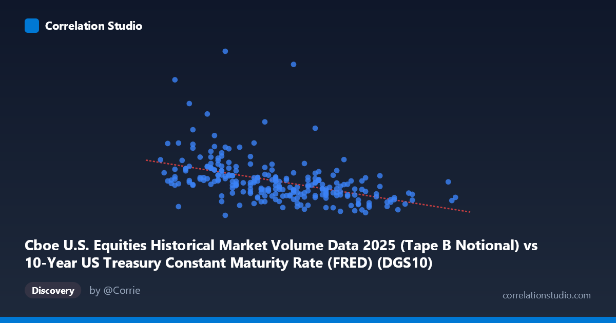
Cboe U.S. Equities Historical Market Volume Data 2025 (Tape B Notional) vs 10-Year US Treasury Constant Maturity Rate (FRED) (DGS10)
- Pearson correlation (r)
- -0.4669
- Spearman correlation
- -0.5933
- p-value
- 0
- Sample size (n)
- 248
- 95% confidence interval
- -0.559 to -0.3635
- Granger causality
- None
- Granger optimal lag
- 10
AI analysis
Analysis of 10-Year Treasury Yield vs. Cboe Tape B Notional Volume
1. What the Visualization Reveals
The scatterplot displays a moderate negative relationship between the 10-year US Treasury constant maturity rate (x-axis) and Cboe Tape B notional trading volume (y-axis) across 248 paired daily observations spanning 2025. As Treasury yields rise, notional equity trading volume on Tape B tends to decline. The linear regression equation (y = -7.19×10⁹x + 3.98×10¹⁰) quantifies this inverse slope, suggesting that each 1 percentage point increase in the 10-year yield is associated with roughly a $7.19 billion decrease in notional volume. Visually, the cloud of points slopes downward from left to right, though with considerable scatter, indicating the relationship is real but far from deterministic.
2. Correlation Strength, Direction, and Statistical Framing
The Pearson r of -0.467 confirms a moderate negative correlation, but the r² of 0.218 is the more practically grounding figure — Treasury yield movements explain only about 21.8% of the variance in Tape B notional volume, leaving roughly 78% unexplained by this variable alone. The 95% confidence interval for r of [-0.559, -0.364] is meaningfully bounded away from zero, and the p-value of 7.77×10⁻¹⁵ leaves no doubt about statistical significance given n=248. However, statistical significance here is partly a function of sample size and should not be conflated with practical magnitude. Critically, the Granger causality tests fail in both directions (X→Y: F=0.728, p=0.697; Y→X: F=0.809, p=0.620), meaning that neither variable reliably predicts the other's future values at the optimal 10-period lag. This is an important caveat: the contemporaneous correlation exists, but there is no temporal predictive leverage to exploit.
3. Notable Patterns, Clusters, and Outliers
Several features stand out in the data. There is a notable cluster of high-yield, lower-volume observations in the x=[4.55–4.79] range, broadly consistent with the negative trend. Conversely, the lower yield range (x=[3.97–4.20]) shows wider vertical dispersion, with some extreme high-volume outliers — for instance, observations around (4.05, ~18.6B) and (4.23, ~13.7B) sit well above the regression line, suggesting episodic spikes in trading activity that yield alone cannot explain. The fact that Spearman ρ exceeds Pearson r is an important diagnostic: it suggests the relationship is monotonic but non-linear, meaning a logarithmic or power-law fit may better characterize how volume responds to yield changes, particularly at the lower end of the yield range where volume variance is highest.
4. Confounding Factors and Interpretive Caveats
Several confounds warrant caution. First, Tape B notional volume is influenced by market microstructure factors, index rebalancing events, earnings seasons, and macro announcements that are entirely independent of yield levels. Second, the dataset covers only 2025, a single calendar year with a relatively narrow yield range (3.97–4.79%), limiting generalizability. Third, causality is ambiguous at best — both variables likely respond to common drivers such as Federal Reserve policy signals, inflation data releases, or risk-off/risk-on sentiment shifts, making this a classic case of spurious correlation via shared confounders rather than a direct mechanism. Fourth, the mislabeled axes in the source data (dataset names appear swapped between axis labels and descriptions) suggest a metadata issue that should be verified before drawing firm conclusions.
5. Actionable Insights and Further Investigation
Given these findings, several paths forward are worth pursuing. Replace linear regression with a logarithmic or polynomial model to better capture the non-linear monotonic relationship flagged by the Spearman diagnostic — this could meaningfully improve explanatory power beyond the current 21.8%. Investigate the high-volume outlier days specifically: identifying whether they coincide with FOMC meetings, CPI releases, or major index events would help disentangle yield-driven volume changes from event-driven spikes. Expanding the dataset to multiple years would test whether this inverse relationship is structurally stable or 2025-specific. Finally, incorporating additional predictors — VIX, equity index returns, bid-ask spreads, or Fed funds futures — into a multivariate model would likely absorb much of the unexplained 78% variance and provide a more actionable forecasting framework.
X dataset: 10-Year US Treasury Constant Maturity Rate (FRED)
Y dataset: Cboe U.S. Equities Historical Market Volume Data 2025
Part of experiment: Daily - 10-Year US Treasury Constant Maturity Rate (FRED) vs Cboe U.S. Equities Historical Market Volume Data 2025