World Bank CO2 Emissions by Country (DataBank) (Solid Fuel) vs US Employment and Unemployment (employed_percent)
- Pearson correlation (r)
- 0.5449
- Spearman correlation
- 0.6959
- p-value
- 0
- Sample size (n)
- 80
- 95% confidence interval
- 0.3694 to 0.6828
- Granger causality
- None
- Granger optimal lag
- 10
- Time coverage
- 1941-01-01 to 2020-01-01
AI analysis
Scatterplot Analysis: Solid Fuel CO2 Emissions vs. US Employment Percentage
1. Overall Relationship Pattern
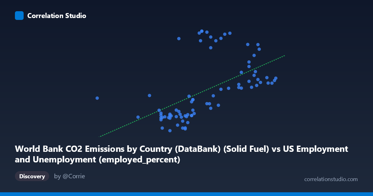
The scatterplot reveals a positive but highly dispersed relationship between World Bank solid fuel CO2 emissions and US employment percentage. While an upward trend is visible in the linear regression line (y = 1214.66x − 53223.7), the data points exhibit enormous vertical scatter across the entire x-range, suggesting that the two variables move loosely in the same direction but are far from tightly coupled. Notably, the x-axis range is relatively compressed (50.40–64.40), while the y-axis spans nearly threefold (≈9,555 to ≈31,154), meaning small differences in solid fuel emissions correspond to wildly varying employment percentages. The visual impression is one of a weak-to-moderate trend buried within substantial noise.
2. Correlation Strength, Direction, and Temporal Predictability
The Pearson r of 0.5449 indicates a moderate positive correlation, but the r² of 0.2969 is the more sobering figure — only ~29.7% of the variance in US employment percentage is explained by solid fuel CO2 emissions, leaving roughly 70% attributable to other factors. The 95% confidence interval for r spans [0.3694, 0.6828], a fairly wide band that reflects meaningful uncertainty, though the p-value of 1.738×10⁻⁷ confirms the correlation is statistically significant well below conventional thresholds and is unlikely to be a chance artifact given n=80 paired observations. Critically, Granger causality testing finds no significant predictive directionality in either direction: X→Y yields F=1.158, p=0.341 and Y→X yields F=1.736, p=0.099, both failing to reach significance even at α=0.10. This means that knowing past values of solid fuel emissions does not meaningfully help predict future US employment rates, and vice versa — the correlation, though statistically present, carries no demonstrated temporal predictive utility at the optimal 10-period lag.
3. Notable Patterns, Clusters, and Outliers
Several structural features stand out in the data:
- Vertical clustering at mid-range x-values (≈56–59): A dense cluster of points in this zone spans nearly the full y-range (≈10,000–31,000), indicating that identical or near-identical emission levels are associated with vastly different employment percentages across different years — a hallmark of a confounded or temporally mixed relationship. - High-y outliers at low-to-mid x-values: Points such as (56.80, 29,528), (58.50, 29,066), (58.60, 31,154), and (59.00, 30,926) sit dramatically above the regression line, suggesting specific historical years where employment surged independently of emission levels. - Low outlier: (50.40, 16,616) represents the minimum x-value yet has a middling y-value, pulling the regression fit leftward. - The Spearman ρ exceeding Pearson r is an important diagnostic — it signals that the true relationship may be non-linear (potentially logarithmic or polynomial), meaning the linear regression model understates the actual association structure and a curved fit might better capture the data's behavior, particularly the apparent plateauing at higher x-values.
4. Confounding Factors and Interpretive Caveats
Several critical caveats undermine any causal interpretation:
- Spurious correlation via shared time trend: Both solid fuel CO2 emissions (globally driven by industrialization) and US employment rates follow long-run secular trends tied to macroeconomic cycles. Over 1941–2020, both variables are influenced by WWII mobilization, post-war expansion, oil shocks, recessions, and deindustrialization — producing correlation without any meaningful mechanistic link. - Dataset mismatch: The x-axis is labeled as coming from the "US Employment and Unemployment" dataset but represents World Bank CO2 data (solid fuel), while the y-axis reverses this pairing. This cross-dataset joining requires careful validation that the annual merge is properly aligned by year. - Aggregation level: World Bank solid fuel emissions are a global aggregate (or country-level), while US employment is a national labor market indicator — these operate at fundamentally different geographic and causal scales. - Non-linearity and heteroscedasticity: The increasing vertical spread at higher x-values suggests heteroscedasticity, violating linear regression assumptions and inflating confidence in the linear model's fit. - Omitted variable bias: GDP growth, energy policy shifts, global recessions, and demographic changes all simultaneously influence both variables and are absent from this bivariate model.
5. Actionable Insights and Further Investigation
Given these findings, several analytical directions are warranted:
1. Test non-linear models: Fit polynomial (quadratic) or logarithmic regression curves given the Spearman Pearson signal; compare AIC/BIC to the linear model to determine whether a non-linear form is justified. 2. Detrend both time series: Apply first-differencing or HP filtering to remove shared secular trends before re-computing correlation — this would reveal whether any cyclical co-movement persists beyond the long-run trend. 3. Extend Granger causality testing with shorter lags: The 10-period optimal lag is quite long; testing lags 1–5 may reveal shorter-term predictive signals that the 10-period model obscures. 4. Segment by era: Split the 1941–2020 period into pre/post-1973 (oil shock), pre/post-1990 (deindustrialization), and pre/post-2008 (financial crisis) subsets to test whether the correlation is structurally stable or driven by a specific historical regime. 5. Introduce control variables: A multivariate regression incorporating GDP growth, energy price indices, and population size would clarify whether any residual solid-fuel–employment association survives after controlling for obvious confounders. At present, the 29.7% explained variance and absent Granger causality provide insufficient grounds for policy inference from this bivariate relationship alone.
X dataset: US Employment and Unemployment
Y dataset: World Bank CO2 Emissions by Country (DataBank)
Part of experiment: Yearly - US Employment and Unemployment vs World Bank CO2 Emissions by Country (DataBank)