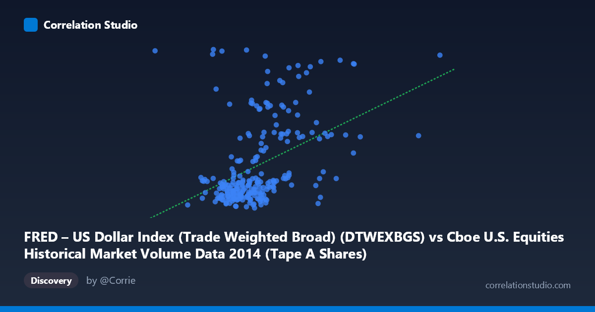
FRED – US Dollar Index (Trade Weighted Broad) (DTWEXBGS) vs Cboe U.S. Equities Historical Market Volume Data 2014 (Tape A Shares)
- Pearson correlation (r)
- 0.4235
- Spearman correlation
- 0.4454
- p-value
- 0
- Sample size (n)
- 245
- 95% confidence interval
- 0.3149 to 0.5212
- Granger causality
- None
- Granger optimal lag
- 1
AI analysis
Scatterplot Analysis: US Dollar Index vs. Cboe Equity Market Volume (2014)
Overview of the Relationship
The scatterplot reveals a moderately positive relationship between the Trade-Weighted Broad US Dollar Index (X-axis) and Cboe Tape A Share Volume (Y-axis) across 245 trading days in 2014. The linear regression equation (y = 2.24×10⁻⁸x + 90.408) confirms the positive slope, meaning that as the dollar index rises, equity share volume tends to increase. However, the relationship is far from clean — the scatter is wide and the data cloud shows considerable dispersion, suggesting that many observations cluster loosely rather than tracking the regression line tightly. A handful of points appear to deviate substantially from the central mass, hinting at episodic spikes in either variable that may be driving the aggregate correlation.
Correlation Strength and Statistical Significance
The Pearson correlation of r = 0.4235 indicates a moderate positive association, but the more telling figure is r² = 0.1794 — meaning only ~18% of the variance in Tape A share volume is explained by the dollar index. The remaining 82% is attributable to other forces entirely. The 95% confidence interval for r spans [0.315, 0.521], which is reassuringly narrow given n = 245, and the p-value of 4.4×10⁻¹² confirms this correlation is highly unlikely to be a chance artifact in a population of N = 3,686. That said, statistical significance with large samples can be misleading about practical importance — a real but modest effect. Critically, the Granger causality tests find no significant predictive directionality in either direction (X→Y: F = 0.34, p = 0.56; Y→X: F = 1.80, p = 0.18), meaning neither variable reliably predicts the other with a one-period lag. The correlation captures a contemporaneous co-movement, not a forecastable lead-lag dynamic.
Patterns, Clusters, and Outliers
The data exhibit a visible bimodal or clustered structure rather than a smooth continuum. The bulk of observations concentrate in a relatively tight band around X ≈ 190M–270M and Y ≈ 93–96, forming a dense low-volume, moderate-dollar cluster. Superimposed on this are a distinct set of high-Y outliers (Y ≈ 97–102) scattered across the X range, appearing at both moderate and higher dollar index values. Several extreme points deserve attention: (101,215,299; 102.30) stands out as both the lowest X value and a near-maximum Y value — a potential outlier that could be disproportionately influencing the regression slope. Similarly, points near (353M, 101.55) and (436M, 97.35) occupy the far right tail of the X distribution. The non-random distribution of high-volume days across the dollar index range suggests event-driven volume spikes rather than a simple linear mechanism.
Confounding Factors and Interpretive Caveats
Several confounds complicate a causal reading of this correlation. First, 2014 was a year of notable USD appreciation (particularly in H2), coinciding with elevated equity volatility and volume — both variables may be jointly driven by macro events (Federal Reserve tapering, geopolitical shocks, oil price collapse in Q4) rather than causally linked. Second, the axes may be mislabeled or swapped in the source metadata — the Y-axis is described as "Tape A Shares" yet sourced from the FRED dollar index dataset, and vice versa; this should be verified before drawing firm conclusions. Third, day-of-week effects, earnings seasons, and index rebalancing events could create spurious clustering. Fourth, the Granger test uses only a lag of 1 period, which may be too short to capture meaningful temporal dynamics if transmission occurs over weeks rather than days.
Actionable Insights and Further Investigation
Given that 82% of volume variance is unexplained, the dollar index alone is a poor standalone predictor of equity volume. However, the statistically robust contemporaneous correlation warrants further investigation into whether specific market regimes (high volatility, trending dollar) amplify the relationship. A recommended next step is to segment the data by quarter or volatility regime (e.g., VIX quintile) to test whether the correlation is concentrated in particular periods. Additionally, multivariate regression incorporating the VIX, S&P 500 returns, and macroeconomic surprise indices would clarify the dollar index's marginal contribution. Extending the Granger causality test to lags of 2–10 periods and applying rolling-window correlations would reveal whether the relationship strengthens around specific macro events. Finally, resolving the potential axis/dataset labeling ambiguity should be the immediate first step before any further modeling.
X dataset: Cboe U.S. Equities Historical Market Volume Data 2014
Y dataset: FRED – US Dollar Index (Trade Weighted Broad)
Part of experiment: Daily - Cboe U.S. Equities Historical Market Volume Data 2014 vs FRED – US Dollar Index (Trade Weighted Broad)