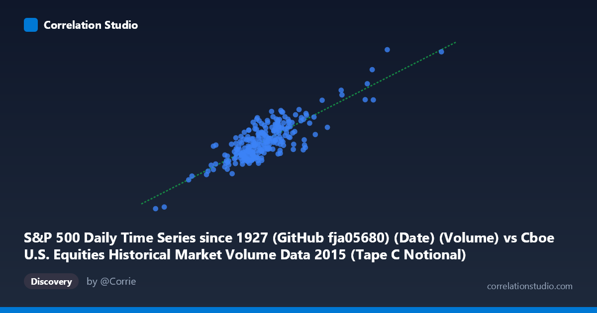
S&P 500 Daily Time Series since 1927 (GitHub fja05680) (Date) (Volume) vs Cboe U.S. Equities Historical Market Volume Data 2015 (Tape C Notional)
- Pearson correlation (r)
- 0.8335
- Spearman correlation
- 0.7344
- p-value
- 0
- Sample size (n)
- 252
- 95% confidence interval
- 0.7914 to 0.8677
- Granger causality
- None
- Granger optimal lag
- 10
- Time coverage
- 2015-01-02 to 2015-12-31
AI analysis
Analysis: S&P 500 Trading Volume vs. Cboe Tape C Notional Value (2015)
Relationship Overview The scatterplot reveals a strong positive linear relationship between S&P 500 daily trading volume (X-axis) and Cboe Tape C notional value (Y-axis) across 252 trading days in 2015. As daily equity trading volume increases, the notional value of trades on Tape C exchanges rises correspondingly. This is an intuitively sensible relationship — higher share volumes traded at prevailing market prices naturally generate larger notional dollar flows. The linear regression equation (y = 0.4598x + 1.006×10⁹) suggests that for every additional unit of volume, notional value increases by roughly $0.46, with a substantial baseline intercept reflecting the structural floor of notional activity even on lower-volume days.
Correlation Strength and Statistical Significance The Pearson correlation of r = 0.8335 is strong, and the coefficient of determination r² = 0.6947 indicates that approximately 69.5% of the variance in Tape C notional value is explained by overall S&P 500 volume — a meaningful but incomplete explanation, leaving ~30.5% attributable to other factors. The 95% confidence interval [0.7914, 0.8677] is narrow and sits firmly in "strong" territory, and with a p-value effectively at zero across 252 paired observations (from a population of 3,302), there is no meaningful statistical uncertainty about the existence of this relationship. However, the Granger causality results are notably inconclusive: neither direction (X→Y: F=0.745, p=0.681; Y→X: F=0.773, p=0.655) achieves significance even at a 10-lag optimal structure. This means that while the two series move together contemporaneously, neither leads the other in a temporally predictive sense — they are co-driven rather than causally sequenced.
Patterns, Clusters, and Outliers The bulk of the data clusters in a dense core between roughly 4.5–6.5 billion in volume and 2.5–4.5 billion in notional value, consistent with typical 2015 market conditions. However, the scatter reveals a meaningful upper-right tail of high-volume, high-notional days — several points exceed 8–9 billion in volume with notional values pushing toward 5–6.8 billion, likely corresponding to August 2015 market volatility events. The single most extreme point (approximately 12.35B volume, 6.68B notional) stands out as a clear outlier and almost certainly represents the August 24, 2015 flash crash, a day of extraordinary market stress and record volume. A modest increase in vertical spread at higher X values hints at slight heteroscedasticity — notional value becomes more variable on high-volume days, possibly because price levels (which multiply volume into notional) fluctuate more dramatically during volatile sessions.
Confounding Factors and Caveats Several important caveats temper interpretation. First, notional value is mechanically linked to both volume AND price, so the correlation partly reflects the fact that high-stress days (high volume) also tend to coincide with elevated intraday price swings, inflating notional independently of volume alone. This creates a compound driver problem. Second, Tape C specifically covers NYSE Arca-listed securities, so the relationship captures only a subset of total market activity — structural shifts in exchange market share during 2015 could influence the relationship. Third, the dataset spans only a single calendar year (2015), which included an unusually sharp volatility episode; the r² and regression slope may not generalize to lower-volatility years. Finally, the Granger non-causality finding (despite the high contemporaneous r) strongly suggests a latent common driver — likely investor sentiment, macroeconomic news, or risk-off events — is simultaneously moving both series rather than one causing the other.
Actionable Insights and Further Investigation Practitioners and researchers should consider decomposing the relationship by volatility regime (e.g., VIX quintiles) to test whether the correlation holds uniformly or strengthens during stress periods. Removing the August 2015 outlier cluster and re-running the regression would clarify whether the observed slope is inflated by tail events. Since Granger causality is absent, using volume alone as a leading indicator for notional flows (or vice versa) in trading models would be unreliable — any predictive model should incorporate exogenous signals such as implied volatility, macroeconomic calendar events, or pre-market futures activity. Extending the analysis across multiple years would help distinguish structural from episodic relationships, and including other Tape designations (A, B) alongside Tape C would reveal whether this correlation is exchange-specific or a broad market phenomenon.
X dataset: Cboe U.S. Equities Historical Market Volume Data 2015
Y dataset: S&P 500 Daily Time Series since 1927 (GitHub fja05680) (Date)
Part of experiment: Daily - Cboe U.S. Equities Historical Market Volume Data 2015 vs S&P 500 Daily Time Series since 1927 (GitHub fja05680) (Date)