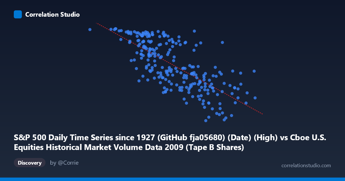
S&P 500 Daily Time Series since 1927 (GitHub fja05680) (Date) (High) vs Cboe U.S. Equities Historical Market Volume Data 2009 (Tape B Shares)
- Pearson correlation (r)
- -0.7318
- Spearman correlation
- -0.7434
- p-value
- 0
- Sample size (n)
- 252
- 95% confidence interval
- -0.7845 to -0.6687
- Granger causality
- Bidirectional
- Granger optimal lag
- 10
AI analysis
Analysis: S&P 500 Daily High vs. Cboe Tape B Share Volume (2009)
Relationship Overview The scatterplot reveals a moderately strong negative relationship between the S&P 500 daily high price (X-axis) and Cboe Tape B share volume (Y-axis) across 2009. As the S&P 500's daily high increases, Tape B share volume tends to decline — a pattern consistent with the broader market narrative of 2009, where the index began the year near crisis lows (with correspondingly elevated trading volumes driven by panic and uncertainty) and recovered substantially through the year (as volatility and volume normalized downward). The linear regression equation y = -1.93×10⁻⁶x + 1239.97 captures this inverse trend, with the steep negative slope reflecting meaningful volume sensitivity to price level changes across the index's wide range (~33.8M to ~255.8M in index-equivalent units).
Correlation Strength and Statistical Robustness The correlation coefficient of r = -0.7318 indicates a strong negative association, and the R² of 0.5356 means that approximately 53.6% of the variance in Tape B share volume is explained by the S&P 500 daily high — a substantial but incomplete explanation, leaving ~46% attributable to other factors. The 95% confidence interval of [-0.7845, -0.6687] is relatively narrow and lies entirely in negative territory, confirming the direction with high confidence. The p-value of essentially zero, combined with a sample of n=252 drawn from N=3,232, provides extremely strong evidence against the null hypothesis of no correlation. Importantly, the Granger causality analysis identifies bidirectional temporal predictive relationships at a 10-period lag: X→Y (F=2.33, p=0.013) and Y→X (F=2.75, p=0.003), with Y→X being slightly stronger. This suggests that not only do higher S&P 500 prices predict lower subsequent Tape B volume, but elevated Tape B volume also provides a forward signal for S&P 500 price direction — consistent with volume as a leading market indicator.
Notable Patterns and Outliers Several features stand out in the data. The scatter shows a broad funnel or heteroscedastic shape, with greater Y-axis dispersion at lower X values (early 2009 crisis period) and tighter clustering at higher X values (late 2009 recovery). This suggests that volume behavior was more unpredictable during market stress. Notably, there is a cluster of high-volume, low-price points in the lower-left region, corresponding to the February–March 2009 market trough, and a distinct cluster of lower-volume, higher-price points in the upper-right representing the recovery. A few potential outliers are visible — particularly the point near (254.5M, ~930) and (225.7M, ~930), which show relatively high prices but higher-than-expected volume, possibly reflecting specific high-activity trading days during the recovery. The point at (33.8M, ~1126) appears anomalous and warrants scrutiny.
Confounding Factors and Caveats Several important caveats apply. Time as a confound is paramount: this is essentially a time-series correlation where both variables are simultaneously driven by the progression from crisis to recovery in 2009, meaning the correlation may largely capture a shared temporal trend rather than a direct causal mechanism. Tape B specifically covers NYSE American (AMEX) and regional exchange tapes, so its volume dynamics may differ from total market volume and may be disproportionately influenced by specific securities or sectors active on those venues. The bidirectional Granger causality, while statistically significant, operates at a 10-day lag and should not be over-interpreted as economic causation — Granger causality detects predictive patterns, not structural mechanisms. Additionally, volatility (VIX), institutional behavior, algorithmic trading patterns, and macro events (TARP, Fed interventions) likely explain much of the residual 46% variance.
Actionable Insights and Further Investigation Practitioners and researchers should consider several next steps. First, decompose the time trend by detrending or differencing both series to test whether the correlation persists beyond the shared 2009 recovery trajectory — a spurious correlation driven purely by trending would weaken substantially after detrending. Second, incorporate VIX or realized volatility as a control variable, since volatility is a known driver of trading volume and would help isolate the price-volume relationship proper. Third, the 10-period Granger lag is practically actionable: a rolling model using lagged Tape B volume as a predictor of near-term S&P 500 direction (and vice versa) could be tested in a trading or risk-monitoring context. Finally, comparing 2009 to other crisis and non-crisis years would reveal whether this inverse price-volume dynamic is a general market property or specific to distressed-market regimes — a finding with significant implications for market microstructure research.
X dataset: Cboe U.S. Equities Historical Market Volume Data 2009
Y dataset: S&P 500 Daily Time Series since 1927 (GitHub fja05680) (Date)
Part of experiment: Daily - Cboe U.S. Equities Historical Market Volume Data 2009 vs S&P 500 Daily Time Series since 1927 (GitHub fja05680) (Date)