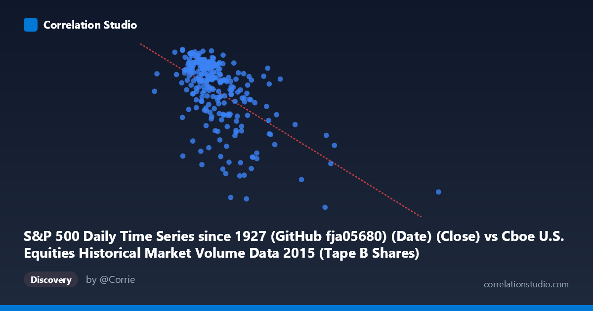
S&P 500 Daily Time Series since 1927 (GitHub fja05680) (Date) (Close) vs Cboe U.S. Equities Historical Market Volume Data 2015 (Tape B Shares)

Pearson correlation (r): -0.5686
Spearman correlation: -0.5448
p-value: 0
Sample size (n): 252
95% confidence interval: -0.6467 to -0.4786
Granger causality: None
Granger optimal lag: 7

AI analysis

Analysis: S&P 500 Close Price vs. Cboe Tape B Share Volume (2015)

Relationship Overview The scatterplot reveals a moderate negative relationship between S&P 500 closing prices (X-axis) and Cboe Tape B share volumes (Y-axis) across 252 trading days in 2015. As the S&P 500 index level increases, Tape B share volume tends to decrease, and conversely, lower index levels are associated with higher trading volumes. This inverse pattern is consistent with a well-documented market behavior: elevated volatility and declining prices tend to drive increased trading activity, while calmer, rising markets often see reduced volume participation. The linear regression equation (y = -1.09×10⁻⁶x + 2173.78) quantifies this slope, showing that each unit increase in the index corresponds to a modest but consistent reduction in Tape B shares traded.

Correlation Strength and Statistical Significance The Pearson correlation of r = -0.5686 indicates a moderate negative association, and the R² of 0.3233 means that approximately 32.3% of the variance in Tape B volume is explained by the S&P 500 price level alone — meaningful, but leaving roughly 68% of variation unexplained by this single predictor. The 95% confidence interval of [-0.6467, -0.4786] is relatively tight and does not cross zero, and the p-value of effectively 0 (given N = 3,302 population size and n = 252 paired observations) confirms this relationship is highly statistically significant and unlikely to be a chance finding. However, the Granger causality results complicate the narrative considerably: neither direction shows significant temporal predictive power (X→Y: F = 1.90, p = 0.070; Y→X: F = 0.52, p = 0.818). This means that despite the clear contemporaneous correlation, past S&P 500 prices do not meaningfully predict future Tape B volumes at a 7-period lag, and vice versa — the relationship is associative rather than directionally predictive in a temporal sense.

Notable Patterns, Clusters, and Outliers Several features stand out in the sample points. The bulk of observations cluster between S&P 500 values of roughly 75M–130M (index close range ~1,950–2,130), forming a dense core with moderate scatter. However, there are notable outliers at the lower-right of the distribution — points such as (205,030,139; 1,867.61) and (213,882,547; 1,970.89) represent days with extremely high volume and low index prices, likely corresponding to the late August 2015 market selloff, a period of sharp volatility and panic selling that drove both elevated volume and depressed prices simultaneously. These high-leverage outliers likely exert disproportionate influence on the regression slope and correlation coefficient. Additionally, a handful of points at moderate X values show unusually high Y values (e.g., ~2,130), suggesting high-price, moderate-volume days typical of quieter bull-market sessions earlier in 2015.

Confounding Factors and Caveats Several important caveats apply to this interpretation. First, both variables are time-indexed, meaning the correlation partly reflects shared temporal trends rather than a pure structural relationship — the S&P 500 declined significantly in August 2015 while volumes spiked, creating a spurious-looking correlation driven largely by a single event window. Second, Tape B specifically covers NYSE American and regional exchange-listed securities, which may respond differently to broad market stress than the full S&P 500 universe, introducing a scope mismatch. Third, the absence of Granger causality suggests the relationship may be contemporaneous and event-driven rather than a stable lead-lag dynamic, undermining its utility for prediction. Finally, omitted variables such as VIX (volatility index), macroeconomic announcements, Federal Reserve communications, and options expiration cycles could independently drive both price levels and volume, acting as common causes that inflate the apparent correlation.

Actionable Insights and Further Investigation Practitioners should avoid using S&P 500 price level alone as a volume predictor given the weak temporal causality and substantial unexplained variance. A more robust model would incorporate implied volatility (VIX) as a co-predictor, since fear-driven volume spikes likely explain much of the August outlier cluster. It would be worth segmenting the analysis by removing or separately analyzing the August–September 2015 volatility episode to determine whether the correlation persists in calmer regimes, or is largely an artifact of that single stress period. Extending the analysis with rolling-window correlations could reveal whether this inverse relationship is stable across time or regime-dependent. Finally, comparing Tape B behavior against Tape A and Tape C volumes under similar conditions would help isolate whether this pattern is exchange-specific or a market-wide phenomenon.

X dataset: Cboe U.S. Equities Historical Market Volume Data 2015

Y dataset: S&P 500 Daily Time Series since 1927 (GitHub fja05680) (Date)

Part of experiment: Daily - Cboe U.S. Equities Historical Market Volume Data 2015 vs S&P 500 Daily Time Series since 1927 (GitHub fja05680) (Date)