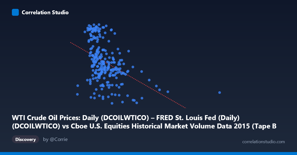
WTI Crude Oil Prices: Daily (DCOILWTICO) – FRED St. Louis Fed (Daily) (DCOILWTICO) vs Cboe U.S. Equities Historical Market Volume Data 2015 (Tape B Trade Count)
- Pearson correlation (r)
- -0.4269
- Spearman correlation
- -0.4443
- p-value
- 0
- Sample size (n)
- 252
- 95% confidence interval
- -0.5229 to -0.3202
- Granger causality
- None
- Granger optimal lag
- 1
AI analysis
Analysis: WTI Crude Oil Prices vs. Cboe Tape B Trade Count (2015)
Relationship Overview
The scatterplot reveals a moderate negative relationship between WTI crude oil prices (X-axis) and Cboe Tape B trade counts (Y-axis) across 252 trading days in 2015. As oil prices increase, trade counts tend to decrease, and conversely, lower oil prices are associated with higher trading activity. The linear regression equation (y = -3.12388E-05x + 58.01) reflects this inverse slope, suggesting that for every $1 increase in WTI price (approximately 10,000 units on the X scale), trade count declines modestly. Visually, the data points form a downward-sloping cloud, though with considerable scatter, indicating the relationship exists but is far from deterministic.
Correlation Strength and Statistical Significance
The Pearson correlation of r = -0.4269 indicates a moderate negative association, but the explanatory power is limited: r² = 0.182, meaning only 18.2% of the variance in Tape B trade counts is explained by WTI crude oil prices. While statistically highly significant (p = 1.395E-12, effectively zero), this near-zero p-value is largely a function of the large population context (N = 3,302) rather than a remarkably strong effect. The 95% confidence interval for r [-0.5229, -0.3202] is reasonably tight and lies entirely in negative territory, confirming the direction of the relationship with confidence, but the width of the interval (~0.20) also reflects non-trivial uncertainty about the true effect size. Critically, the Granger causality results show no significant predictive directionality in either direction — neither X→Y (F = 0.1685, p = 0.682) nor Y→X (F = 0.6430, p = 0.423) — meaning that past oil prices do not help predict future trade counts, and vice versa. This strongly cautions against any causal or leading-indicator interpretation.
Patterns, Clusters, and Outliers
Several structural features are visible in the data. There appears to be a dense cluster of points in the lower X range (roughly 130,000–350,000), where trade counts span a wide range from ~37 to ~61, creating significant vertical dispersion. At higher oil price values (X 500,000), the data becomes sparser with trade counts consistently compressed in the 39–47 range, suggesting reduced volatility or a floor effect at elevated prices. A small number of potential outliers exist at the upper X extreme — points near 621,009 and 640,679 with relatively low trade counts (~40) — which may disproportionately influence the regression slope. Additionally, sample points like (309,219, 60.93) and (362,552, 58.34) appear to sit above the regression line in the mid-X range, suggesting local deviations from the linear trend. The relationship may have non-linear characteristics, with a steeper decline at lower price ranges tapering off at higher values.
Confounding Factors and Caveats
Several important caveats temper interpretation. First, 2015 was a structurally unique year for oil markets — WTI prices fell dramatically from ~$55/barrel in January to ~$35/barrel by year-end due to OPEC supply decisions and oversupply concerns, meaning the oil price variable is partly acting as a proxy for calendar time rather than an independent economic signal. Higher trade activity at lower prices may simply reflect increased market volatility and uncertainty during the oil price collapse, which independently drives equity trading volume regardless of the price level itself. Second, Tape B trade counts reflect a specific subset of U.S. equity exchange activity and may be influenced by market structure changes, algorithmic trading patterns, and exchange-specific routing decisions unrelated to commodity prices. Third, the axes in the provided data appear to have dataset labels swapped in the axis descriptions (the X-axis description references Cboe volume data while the Y-axis description references oil price data), which warrants verification before drawing firm conclusions. Finally, the absence of Granger causality at lag-1 suggests any correlation may be contemporaneous or spurious, driven by a common underlying factor such as macroeconomic uncertainty.
Actionable Insights and Further Investigation
Despite the moderate and statistically significant correlation, the low r² and absent Granger causality suggest this relationship has limited practical utility for forecasting or trading strategy. Several avenues merit further investigation: (1) Decompose the time trend by detrending both series to determine whether the correlation persists after removing the shared downward trajectory of 2015, which would test whether this is a genuine relationship or a spurious co-movement; (2) Test non-linear models (e.g., logarithmic or piecewise regression) given the apparent compression of trade counts at higher price levels; (3) Introduce volatility measures (e.g., VIX, oil implied volatility) as intermediary variables to test whether uncertainty — not price level — is the true driver of elevated trade counts; (4) Extend the analysis across multiple years to assess whether 2015 represents a structurally anomalous period; and (5) Examine other Tape segments (Tape A, C) to determine whether this relationship is specific to Tape B or reflects a broader equity market phenomenon.
X dataset: Cboe U.S. Equities Historical Market Volume Data 2015
Y dataset: WTI Crude Oil Prices: Daily (DCOILWTICO) – FRED St. Louis Fed (Daily)
Part of experiment: Daily - Cboe U.S. Equities Historical Market Volume Data 2015 vs WTI Crude Oil Prices: Daily (DCOILWTICO) – FRED St. Louis Fed (Daily)