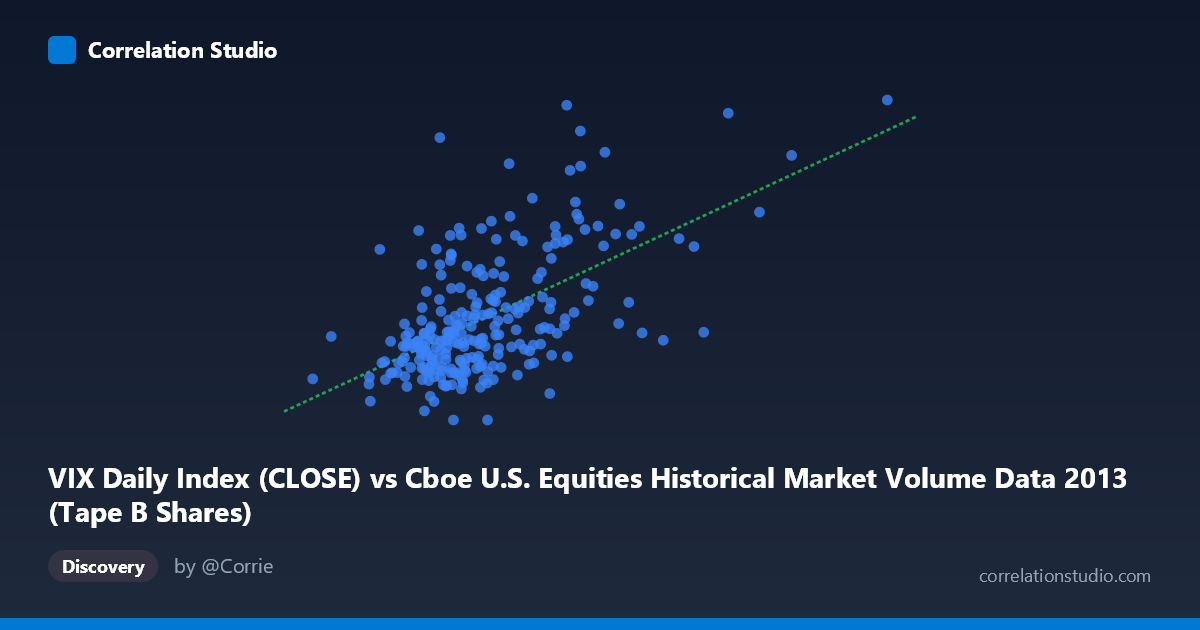
VIX Daily Index (CLOSE) vs Cboe U.S. Equities Historical Market Volume Data 2013 (Tape B Shares)

Pearson correlation (r): 0.5831
Spearman correlation: 0.5179
p-value: 0
Sample size (n): 252
95% confidence interval: 0.4952 to 0.6592
Granger causality: None
Granger optimal lag: 1

AI analysis

Scatterplot Analysis: VIX Daily Index vs. Tape B Shares (2013)

Relationship Overview The scatterplot reveals a moderate positive relationship between the Cboe VIX Daily Index (Close) and Tape B Shares volume for U.S. equities in 2013. As VIX values increase — indicating higher market volatility expectations — Tape B share volumes tend to rise correspondingly. This is economically intuitive: elevated fear or uncertainty in markets typically drives increased trading activity across exchanges. The linear regression equation (y = 5.717e-08x + 10.19) confirms this upward slope, with the intercept suggesting a baseline VIX level of roughly 10.2 even at minimal volume, broadly consistent with the historically low volatility environment of 2013.

Correlation Strength and Statistical Significance The Pearson correlation of r = 0.583 indicates a moderate positive association, with r² = 0.340 meaning that approximately 34% of the variance in VIX levels is explained by Tape B share volume. While statistically robust — the p-value is effectively zero and the 95% confidence interval [0.4952, 0.6592] is comfortably above zero — the remaining 66% of variance is driven by other factors entirely. This means the relationship, though real and meaningful, is far from deterministic. Critically, Granger causality tests reveal no significant temporal predictive direction in either direction (X→Y: F = 0.58, p = 0.447; Y→X: F = 0.28, p = 0.598). This is a pivotal finding: even though the variables co-move, neither reliably predicts the other's future values at a one-period lag, cautioning strongly against any causal or leading-indicator interpretation.

Notable Patterns, Clusters, and Outliers The data cloud displays a clear concentration of points in the lower-left region, roughly where X (volume) falls between 55M–85M and Y (VIX) sits between 12–16, reflecting the dominant low-volatility, moderate-volume trading regime of 2013. Several notable outliers are visible in the upper portions of the chart: points such as (89.9M, 20.34) and (81.8M, 17.67) stand apart from the main cluster with elevated VIX readings, likely corresponding to discrete market stress events during the year (e.g., the May–June taper tantrum). Similarly, the point near (119.7M, 16.28) and (135.0M, 17.27) represent unusually high-volume days. There is also a suggestion of non-linearity or heteroscedasticity: the spread of VIX values widens noticeably as volume increases, implying the relationship may not be uniformly linear across the full range, with high-volume days showing far more VIX variability than low-volume days.

Confounding Factors and Caveats Several important caveats apply. First, the axis labels appear to be swapped relative to what would be typical modeling convention — VIX is conventionally treated as an independent market sentiment indicator, yet here it appears on the X-axis while Tape B Shares (a volume measure) is on the Y-axis, which warrants verification of data mapping. Second, both variables are likely driven by common underlying factors such as macroeconomic announcements, Federal Reserve communications, or geopolitical events, making the observed correlation largely a product of shared confounders rather than a direct causal link. Third, Tape B specifically covers NYSE American and regional exchange stocks, which may not represent the full market, introducing selection bias. Finally, the dataset covers only 2013 — a structurally unusual year with historically suppressed volatility — limiting generalizability.

Actionable Insights and Further Investigation Given the moderate but causally ambiguous correlation, practitioners should avoid using volume alone as a VIX predictor. Instead, further investigation should: (1) test for non-linear models (e.g., logarithmic or polynomial regression) to better capture the heteroscedastic spread at higher volumes; (2) incorporate additional lags beyond one period in Granger causality testing, as market feedback loops may operate over weekly rather than daily horizons; (3) control for known event days (FOMC meetings, earnings seasons, index rebalancing) to isolate whether the correlation is event-driven rather than structural; and (4) replicate the analysis across multiple years to determine whether the 0.583 correlation is specific to 2013's unique low-volatility regime or reflects a more durable market microstructure relationship. A multivariate model incorporating Tape A and Tape C volumes alongside macroeconomic indicators would likely explain substantially more of the remaining 66% variance.

X dataset: Cboe U.S. Equities Historical Market Volume Data 2013

Y dataset: VIX Daily Index

Part of experiment: Daily - Cboe U.S. Equities Historical Market Volume Data 2013 vs VIX Daily Index