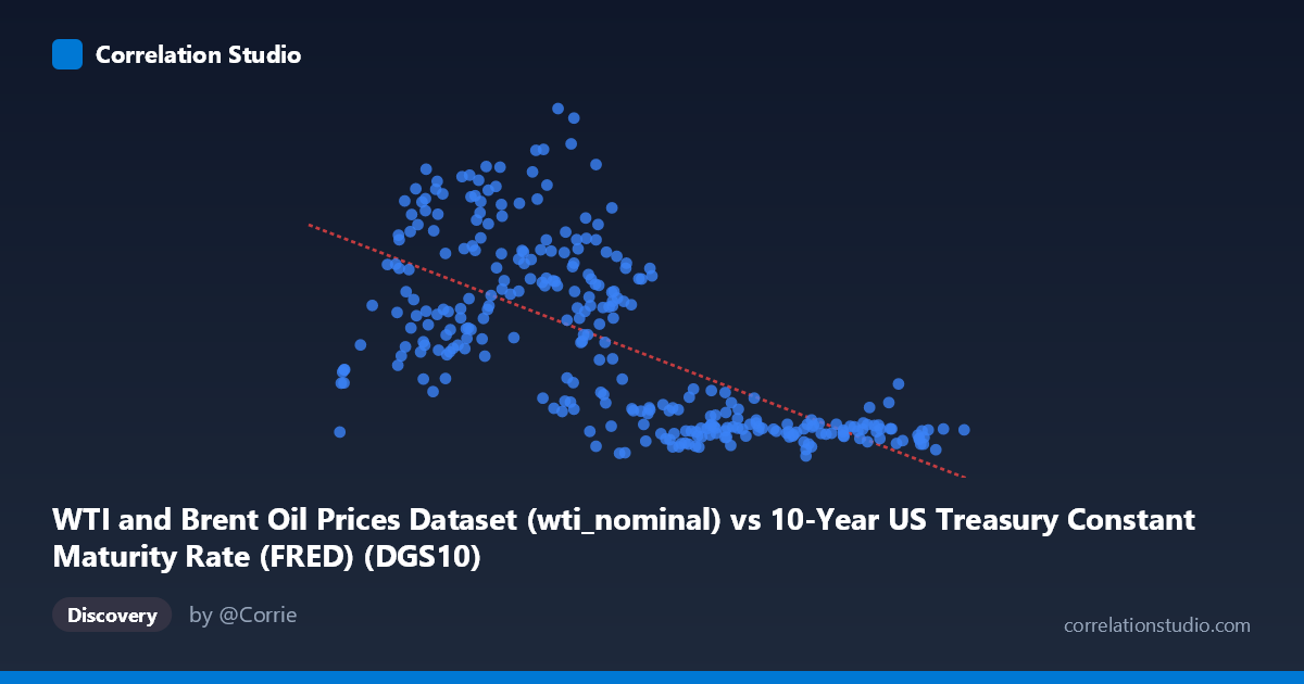
WTI and Brent Oil Prices Dataset (wti_nominal) vs 10-Year US Treasury Constant Maturity Rate (FRED) (DGS10)
- Pearson correlation (r)
- -0.6702
- Spearman correlation
- -0.7094
- p-value
- 0
- Sample size (n)
- 306
- 95% confidence interval
- -0.7276 to -0.6034
- Granger causality
- None
- Granger optimal lag
- 7
AI analysis
Analysis: 10-Year Treasury Yield vs. Real WTI Crude Oil Prices (1986–2026)
Relationship Overview The scatterplot reveals a moderate negative relationship between the 10-year US Treasury constant maturity yield (X-axis) and real (CPI-adjusted) WTI crude oil prices (Y-axis). The linear regression equation — y = -8.90x + 90.01 — indicates that for each 1-percentage-point increase in the Treasury yield, real oil prices are associated with a decline of approximately $8.90 per barrel. Visually, the data show a downward-sloping trend, though with considerable scatter throughout, suggesting the relationship is real but far from deterministic. Notably, the sample points highlight a striking pattern: low Treasury yields (1–3%) tend to coincide with a wide range of oil prices, including many high values (60–127), while higher yields (6–9%) cluster tightly at lower oil prices (roughly 15–35), suggesting potential asymmetry or heteroscedasticity in the relationship.
Correlation Strength and Statistical Significance The Pearson correlation of r = -0.67 indicates a moderate-to-strong negative association, and the R² of 0.449 means that approximately 44.9% of the variance in real oil prices is explained by Treasury yields — a meaningful but incomplete explanation, leaving over half the variance attributable to other factors. The 95% confidence interval of [-0.73, -0.60] is relatively tight and does not include zero, and the p-value of effectively 0 (across n = 306 paired observations) confirms this correlation is highly statistically significant and unlikely to be a chance finding. However, the Granger causality tests are non-significant in both directions (X→Y: F = 0.39, p = 0.91; Y→X: F = 1.10, p = 0.36) at the optimal 7-period lag, meaning neither variable reliably predicts the other temporally. This important caveat distinguishes contemporaneous correlation from causal or predictive dynamics — the two variables move together over time, but neither leads the other in a statistically meaningful way.
Notable Patterns, Clusters, and Non-Linearity The scatterplot displays several noteworthy structural features. There appears to be a dense cluster of points at low yields (0.6–3%) with high oil price variance, reflecting the post-2008 and post-2020 low-rate environments when oil prices swung dramatically due to supply shocks (e.g., the 2020 COVID crash and 2022 spike). Conversely, points at yields above 6% (largely pre-2000 data) show consistently low real oil prices, forming a tight band. This asymmetry hints at possible non-linearity — the relationship may be stronger at certain yield regimes. A few potential outliers exist at low X values with very high Y values (e.g., ~2.94, 107.76 and ~3.46, 113.39), likely corresponding to the 2011–2014 high oil price era. The pattern may be better captured by a curvilinear or piecewise model than a single linear fit.
Confounding Factors and Interpretive Caveats Several important confounders complicate interpretation. First, both variables are heavily influenced by macroeconomic cycles — recessions, inflation regimes, and monetary policy phases — meaning their co-movement may largely reflect shared exposure to broader economic conditions rather than a direct link. Second, the real oil price adjustment (CPI-deflation) and the nominal Treasury yield are not measured on the same inflation-adjusted basis, which could introduce systematic bias. Third, the dataset spans 40 years (1986–2026), a period of dramatically shifting structural regimes (the Great Moderation, the financialization of commodities, zero lower bound policy, and the post-COVID inflation surge), which may violate the stationarity assumptions underlying both correlation and Granger tests. Finally, reverse causality and omitted variables — such as the US dollar strength, global demand cycles, OPEC supply policy, and Federal Reserve forward guidance — are plausible confounders that the bivariate analysis cannot isolate.
Actionable Insights and Further Investigation Given the moderate explanatory power (R² ≈ 0.45) and the absence of Granger causality, practitioners should treat Treasury yields as a concurrent indicator rather than a predictor of oil price direction. For further investigation, it would be valuable to: (1) test for structural breaks (e.g., pre/post-2008) to assess whether the relationship has changed across monetary regimes; (2) apply a multiple regression framework incorporating the US dollar index, global GDP growth, and OPEC production data to better isolate the Treasury yield effect; (3) explore non-linear models (e.g., polynomial regression or regime-switching models) given the apparent heteroscedasticity; and (4) examine whether inflation expectations (e.g., TIPS breakeven rates) mediate the relationship, since both oil prices and nominal yields respond strongly to inflation dynamics. A vector autoregression (VAR) model with additional controls could provide sharper insight into temporal dynamics beyond the bivariate Granger framework used here.
X dataset: 10-Year US Treasury Constant Maturity Rate (FRED)
Y dataset: WTI and Brent Oil Prices Dataset
Part of experiment: Daily - 10-Year US Treasury Constant Maturity Rate (FRED) vs WTI and Brent Oil Prices Dataset