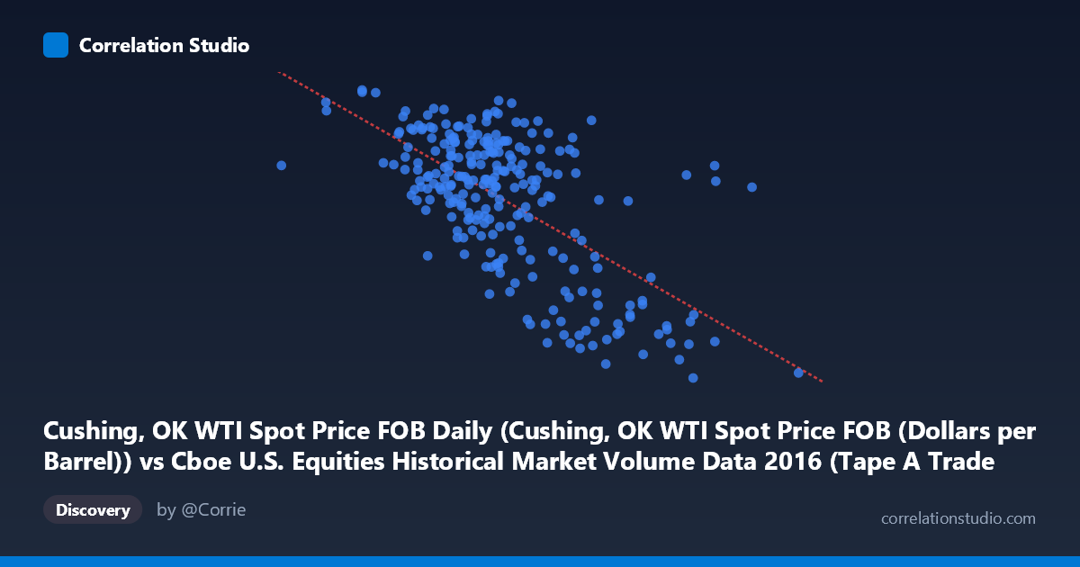
Cushing, OK WTI Spot Price FOB Daily (Cushing, OK WTI Spot Price FOB (Dollars per Barrel)) vs Cboe U.S. Equities Historical Market Volume Data 2016 (Tape A Trade Count)
- Pearson correlation (r)
- -0.6419
- Spearman correlation
- -0.5425
- p-value
- 0
- Sample size (n)
- 252
- 95% confidence interval
- -0.7092 to -0.563
- Granger causality
- None
- Granger optimal lag
- 1
AI analysis
Analysis: WTI Crude Oil Prices vs. Cboe Tape A Trade Count (2016)
Relationship Overview The scatterplot reveals a moderate negative relationship between WTI crude oil spot prices (X-axis) and Cboe Tape A trade counts (Y-axis) across 252 trading days in 2016. As oil prices increase, equity trade counts on Tape A tend to decline, suggesting that higher oil prices coincide with reduced trading activity in this market segment. The linear regression equation (y = −1.456×10⁻⁵x + 63.51) confirms this inverse slope, though the scatter around the regression line is considerable, indicating meaningful unexplained variability.
Correlation Strength and Statistical Framing The Pearson correlation of r = −0.642 reflects a moderate-to-strong negative association. The R² of 0.412 means that roughly 41% of the variance in Tape A trade counts is explained by WTI price levels — a practically meaningful share, but equally notable is the 59% of variance left unexplained, pointing to other influential drivers. The 95% confidence interval of [−0.709, −0.563] is entirely negative and relatively tight, lending confidence that this inverse relationship is genuine and not an artifact of sampling. The p-value of effectively zero confirms high statistical significance given the sample size. However, the Granger causality tests yield no significant directional predictability in either direction (X→Y: F=0.33, p=0.56; Y→X: F=1.12, p=0.29), meaning that while the two variables are contemporaneously correlated, neither reliably predicts future values of the other at a one-period lag. This is a critical distinction: correlation here is not accompanied by temporal forecasting power.
Notable Patterns and Outliers The sample points reveal a distinct cluster of observations where oil prices fall in the roughly 1,100,000–1,450,000 range (in the dataset's units) and trade counts concentrate between ~44 and ~51, forming the dense core of the distribution. There are several notable low-trade-count outliers at high oil price values — points near (2,013,606, 29.55), (1,860,056, 33.21), and (1,726,299, 31.62) — which anchor the negative slope strongly and may represent specific high-price episodes with suppressed trading. Conversely, points like (1,000,524, 51.44) and (1,428,849, 50.90) represent high trade activity at lower price levels. There is also a hint of non-linearity: the relationship appears steeper at higher price ranges and somewhat flatter at lower prices, suggesting a potential curve or threshold effect rather than a purely linear dynamic.
Confounding Factors and Caveats Several important caveats temper interpretation. Temporal autocorrelation is likely in both time series — oil prices and trading volumes trend over days and weeks — meaning observations are not fully independent, which can inflate the apparent significance of the correlation. The year 2016 was atypical, featuring oil price recovery from multi-year lows, post-Brexit volatility, and U.S. election uncertainty, all of which could simultaneously depress oil prices and elevate trading volumes early in the year, creating a spurious or context-specific correlation. The axes may be mislabeled in the dataset metadata (the hint suggests a possible column swap between datasets), warranting verification before drawing firm conclusions. Additionally, macroeconomic regime shifts, risk-off/risk-on sentiment, and seasonal trading patterns could act as common drivers of both variables, making it difficult to isolate any direct causal mechanism.
Actionable Insights and Further Investigation Despite the absence of Granger causality, the 41% shared variance warrants further exploration. Analysts should consider: (1) controlling for broader market volatility (e.g., VIX) and macroeconomic indicators to isolate whether the oil-volume relationship persists independently; (2) testing longer lag structures beyond one period, as Granger tests here used only one lag, potentially missing delayed effects; (3) segmenting the analysis by sub-period (e.g., Q1 vs. Q4 2016) to test whether the correlation is stable or driven by a specific market episode; and (4) examining non-linear regression models given the visual clustering pattern. For practitioners, the lack of Granger causality means oil prices should not be used naively as a leading indicator for Tape A trading volume in algorithmic strategies without substantially more robust modeling.
X dataset: Cboe U.S. Equities Historical Market Volume Data 2016
Y dataset: Cushing, OK WTI Spot Price FOB Daily
Part of experiment: Daily - Cboe U.S. Equities Historical Market Volume Data 2016 vs Cushing, OK WTI Spot Price FOB Daily