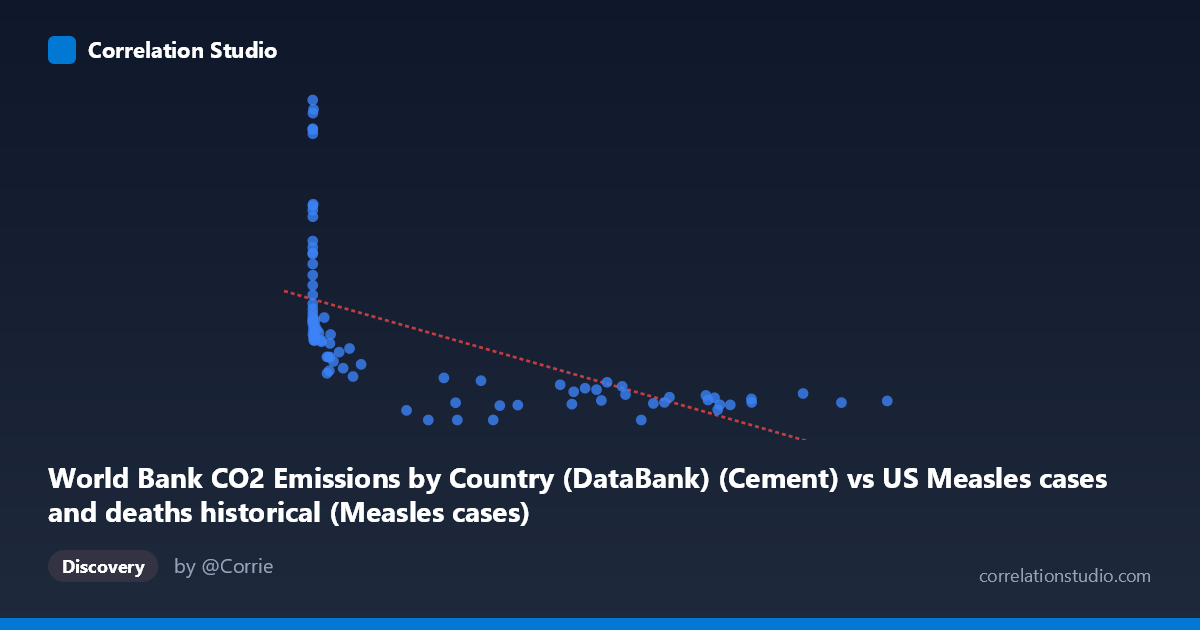
World Bank CO2 Emissions by Country (DataBank) (Cement) vs US Measles cases and deaths historical (Measles cases)
- Pearson correlation (r)
- -0.5975
- Spearman correlation
- -0.8943
- p-value
- 0
- Sample size (n)
- 87
- 95% confidence interval
- -0.7178 to -0.4425
- Granger causality
- None
- Granger optimal lag
- 10
- Time coverage
- 1919-01-01 to 2020-01-01
- Recomputed on refreshed data
- 2026-10-17 (r was -0.5975)
AI analysis
Scatterplot Analysis: Cement CO2 Emissions vs. US Measles Cases
1. Overall Relationship Revealed
The scatterplot reveals a negative association between global cement CO2 emissions and US measles case counts across the 1919–2020 time period. As cement emissions increase (moving right along the X-axis), measles cases tend to decrease, forming a broad downward-sloping cloud. However, the relationship is far from clean — there is substantial vertical spread at low X values, with measles cases ranging from near zero to over 2,600 when cement emissions are small, while high cement emission values cluster at lower measles counts. This asymmetric dispersion strongly hints at a non-linear, likely logarithmic or hyperbolic structure rather than a simple linear one, consistent with the note that Spearman ρ exceeds Pearson r.
2. Correlation Strength, Direction, and Causality
The Pearson correlation of r = -0.5975 indicates a moderate negative relationship, but the explanatory power is more sobering: R² = 0.357, meaning cement CO2 emissions statistically account for only about 35.7% of the variance in US measles cases, leaving nearly two-thirds of the variation unexplained by this model. The 95% confidence interval of [-0.718, -0.443] is moderately wide, reflecting genuine uncertainty in the estimate, though the entire interval sits firmly in negative territory. The p-value of 1.003×10⁻⁹ confirms the correlation is highly statistically significant — this is not a chance finding given n = 87 paired observations. Critically, however, the Granger causality analysis finds no significant predictive direction in either direction (X→Y: F=1.45, p=0.18; Y→X: F=0.77, p=0.66), meaning that past values of cement emissions do not help predict future measles cases and vice versa. This is a strong signal that the correlation is spurious or driven by a shared third variable — most likely the passage of time itself.
3. Notable Patterns, Clusters, and Outliers
Several features stand out visually: - High-leverage outliers at low X values: Points such as (13, 2608.93), (86, 2374.89), (120, 2367.58), (191, 2333.75), and (1274, 2532.94) represent early decades when cement emissions were minimal but measles cases were extremely high, pulling the regression line strongly. - A dense cluster in the mid-to-high X range (roughly 200,000–900,000 units) where measles cases are uniformly low (0–400), suggesting a floor effect possibly tied to vaccination-era elimination of measles in the US. - Three zero-measles observations at moderate-to-high cement values (225,027; 179,829; 280,930), consistent with post-elimination reporting. - The right tail of the X distribution is very sparse and stretched, with values up to 894,134, indicating skewed cement emission growth in recent decades.
4. Confounding Factors and Critical Caveats
This correlation is almost certainly a classic spurious time-series correlation driven by the shared temporal trend of two independently evolving variables. Cement CO2 emissions have grown monotonically with industrialization over the 20th century, while US measles cases collapsed due to the introduction of the measles vaccine in 1963 — a discrete public health intervention with no mechanistic connection to cement production. Both variables are thus co-trending over time, producing a mathematical correlation that implies no causal link whatsoever. Additional confounders include population growth, improved reporting systems, changes in disease surveillance methodology, and global economic development affecting both industrial output and healthcare infrastructure simultaneously. The dataset label mismatch (axes appear to have swapped dataset descriptions) also warrants careful verification before drawing any conclusions.
5. Actionable Insights and Further Investigation
Given the near-certain spuriousness of this correlation, the most productive next steps would be: - Detrend both time series (e.g., first-differencing or residualization against year) before recalculating correlation to remove the shared temporal trend and test whether any residual relationship persists. - Introduce vaccination coverage rates as a covariate to properly model the measles decline and isolate whether any independent signal from emissions remains. - Fit a logarithmic regression model (suggested by Spearman ρ Pearson r) to better capture the non-linear shape of the data cloud and compare AIC/BIC against the linear fit. - Segment the analysis pre- and post-1963 (vaccine introduction) to test whether the correlation structure differs meaningfully across eras. - This dataset pairing serves as an instructive cautionary example for teaching spurious correlations in introductory statistics or data literacy contexts.
X dataset: US Measles cases and deaths historical
Y dataset: World Bank CO2 Emissions by Country (DataBank)
Part of experiment: Yearly - US Measles cases and deaths historical vs World Bank CO2 Emissions by Country (DataBank)