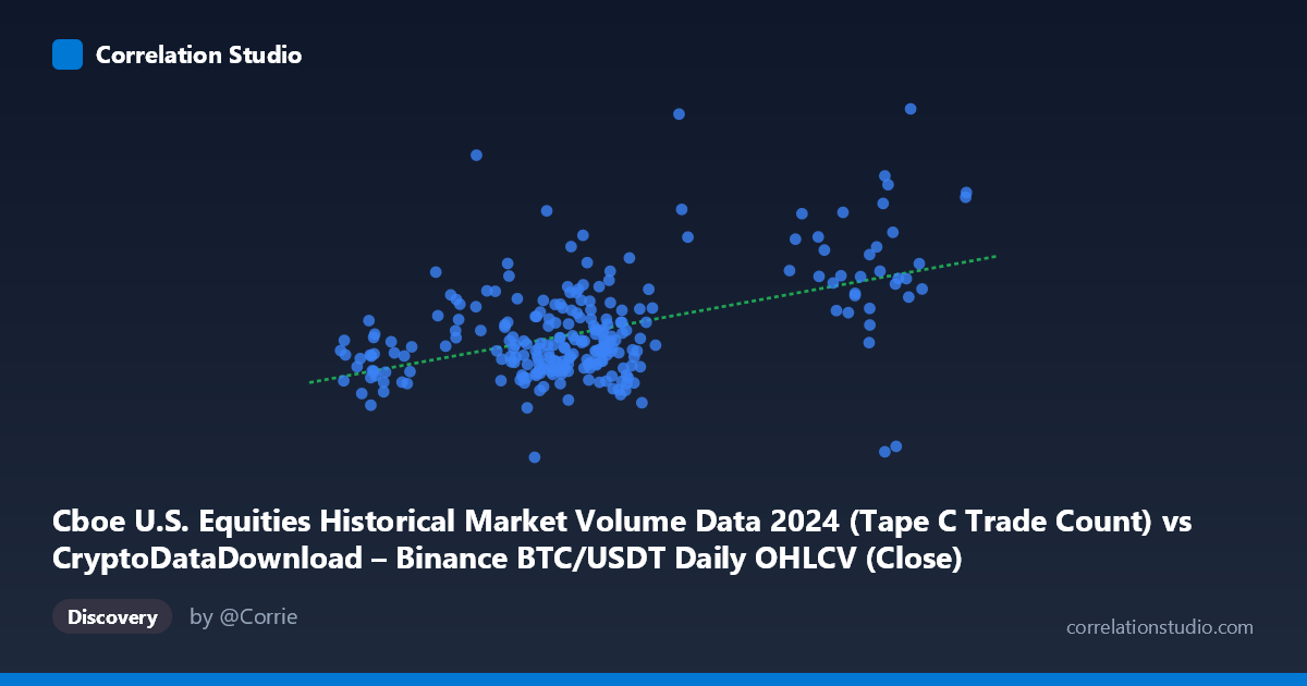
Cboe U.S. Equities Historical Market Volume Data 2024 (Tape C Trade Count) vs CryptoDataDownload – Binance BTC/USDT Daily OHLCV (Close)

Pearson correlation (r): 0.4832
Spearman correlation: 0.3493
p-value: 0
Sample size (n): 252
95% confidence interval: 0.3825 to 0.5726
Granger causality: None
Granger optimal lag: 10
Time coverage: 2024-01-02 to 2024-12-31

AI analysis

Analysis: Cboe Equities Trade Count vs. BTC/USDT Close Price

1. What the Visualization Reveals

The scatterplot shows a moderate positive linear relationship between Tape C trade counts on Cboe U.S. equities and Binance BTC/USDT daily closing prices. Most observations cluster tightly in the X range of ~55,000–72,000 trades, with Y values scattered broadly between roughly $1.6M–$2.4M. A smaller number of points extend the X range out to ~95,000–106,000, and these higher-volume days do not show a dramatically different Y pattern, suggesting the relationship weakens or becomes noisier at the extremes. The overall shape is a loose, upward-sloping cloud rather than a tight linear band — consistent with a real but modest association rather than a deterministic one.

2. Strength, Direction, and Predictive Value

The correlation coefficient (r = 0.483) indicates a moderate positive relationship, with the 95% CI [0.38, 0.57] being fairly narrow and entirely positive — this correlation is statistically robust (p = 4.44E-16), not a fluke of sampling. However, r² = 0.2335 tells the more important practical story: only about 23% of the variance in BTC closing price is explained by equity trade counts, leaving over 76% attributable to other factors. This is a meaningful but far from dominant relationship — useful as one input among many, not a standalone predictor. Critically, the Granger causality tests show no significant predictive direction in either direction (X→Y: p=0.23; Y→X: p=0.50). This means that despite the contemporaneous correlation, past values of one series do not help forecast future values of the other at the tested lag (10 periods). The relationship appears to be a same-period co-movement rather than a lead-lag causal pattern — likely both series are responding to shared macro conditions rather than one driving the other.

3. Notable Patterns and Outliers

Several outliers stand apart: the point at (60208.58, 1,260,223.79) sits far below the main cluster — the lowest Y value in the dataset — while (54018.81, 2,801,223.32) is a high-Y outlier at relatively low X. There's also a subgroup of high-X points (95,849–106,133) that appear to behave differently, with Y values not proportionally elevated (e.g., 98,663.58 → 1,316,054.68, actually one of the lowest Y values despite high X). This suggests a possible ceiling effect or regime change at high trade-count levels, undermining a simple linear model there. The bulk of the data (X between 55K–72K) drives most of the correlation, and the relationship may be more idiosyncratic/noisy within that dense cluster than the aggregate r suggests.

4. Confounding Factors and Caveats

This pairing is unusual: it compares equity market microstructure (trade counts on Cboe, a U.S. stock exchange venue) with a crypto asset price (BTC/USDT on Binance). Any correlation is almost certainly driven by shared macro drivers — overall market risk sentiment, liquidity conditions, volatility regimes, or seasonal/calendar effects (e.g., both trade counts and crypto prices may rise during risk-on periods or major news events) — rather than a direct mechanical link. Trade count is also a volume/activity metric, not a price metric, making this a cross-domain, cross-unit comparison prone to spurious correlation from trending behavior over the year (both series may simply have grown or drifted over 2024 due to unrelated reasons). Additionally, daily data introduces autocorrelation within each series that can inflate apparent correlation strength beyond what independent daily observations would show.

5. Suggestions for Further Investigation

Given the lack of Granger causality, this correlation should not be used for short-term forecasting in either direction. Useful next steps: (a) test for a common latent driver (e.g., VIX, overall market volume, macro risk indices) that might explain co-movement; (b) de-trend both series (e.g., via differencing or detrended residuals) to check if the correlation persists after removing shared drift, since 23% variance explained on raw levels can shrink significantly after detrending; (c) segment the analysis by regime (high vs. low trade-count days) to test the apparent non-linearity/ceiling effect at the high end; and (d) test alternative lag structures and non-linear causality methods (e.g., transfer entropy) given that Granger causality at lag 10 may miss shorter or longer dependency structures.

X dataset: CryptoDataDownload – Binance BTC/USDT Daily OHLCV

Y dataset: Cboe U.S. Equities Historical Market Volume Data 2024

Part of experiment: Bitcoin - CryptoDataDownload – Binance BTC/USDT Daily OHLCV vs Cboe U.S. Equities Historical Market Volume Data 2024