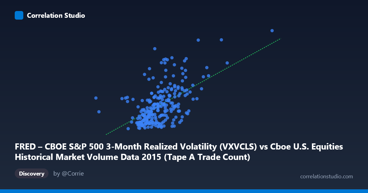
FRED – CBOE S&P 500 3-Month Realized Volatility (VXVCLS) vs Cboe U.S. Equities Historical Market Volume Data 2015 (Tape A Trade Count)
- Pearson correlation (r)
- 0.5579
- Spearman correlation
- 0.5346
- p-value
- 0
- Sample size (n)
- 252
- 95% confidence interval
- 0.4665 to 0.6375
- Granger causality
- None
- Granger optimal lag
- 1
AI analysis
Analysis: CBOE S&P 500 3-Month Realized Volatility vs. Tape A Trade Count (2015)
Relationship Overview The scatterplot reveals a moderate positive relationship between CBOE S&P 500 3-month realized volatility (VXVCLS) and Tape A trade count across U.S. equity exchanges in 2015. The linear regression equation (y = 7.018×10⁻⁶x + 8.477) confirms that as market volume (trade count) increases, realized volatility tends to rise as well. This is conceptually intuitive: higher trading activity is often associated with more uncertain or turbulent market conditions, as participants react to new information, hedge positions, or engage in momentum-driven behavior. The relationship is broadly consistent across the year's trading days, though with meaningful dispersion around the trend line.
Correlation Strength and Statistical Significance The Pearson correlation of r = 0.558 indicates a moderate positive association, but the more telling figure is r² = 0.311 — meaning only 31.1% of the variance in 3-month realized volatility is explained by Tape A trade count. The remaining ~69% is attributable to other factors not captured in this bivariate model. The 95% confidence interval for r ([0.467, 0.638]) is reasonably tight given n = 252 paired observations, and the p-value of effectively zero confirms the relationship is highly statistically significant and not a chance artifact. However, Granger causality tests tell a more cautionary story: neither direction (X→Y or Y→X) is statistically significant at lag 1 (F = 0.063, p = 0.802 for X→Y; F = 0.378, p = 0.539 for Y→X). This means that while the two series are contemporaneously correlated, neither variable reliably predicts the other in the next period — the relationship is associative, not temporally directional in any exploitable sense.
Notable Patterns, Clusters, and Outliers The data exhibits a relatively dense central cluster between trade counts of roughly 1.1M–1.6M and volatility values of 15–22, which likely represents typical market-day conditions during calmer stretches of 2015. However, there is a visible upper-right dispersion of points — notably including values near (2,247,816; 29.58) and (1,778,857; 26.38) — where both variables spike simultaneously, consistent with known volatility events in 2015 (e.g., the August market correction). The point at (576,208; 19.69) is a striking left-side outlier with unusually low trade count but moderate volatility, potentially reflecting a holiday-shortened trading session or a data anomaly. The spread around the regression line widens noticeably at higher trade counts, suggesting heteroscedasticity — the relationship becomes less precise as volumes increase.
Confounding Factors and Caveats Several important caveats apply. First, the axes as described in the metadata appear inverted in labeling — VXVCLS is listed as the X-axis variable but described as deriving from the Cboe market volume dataset, and vice versa; this warrants careful verification before drawing directional conclusions. Second, both variables are likely driven by common underlying factors — major macro events, earnings seasons, Federal Reserve announcements, and geopolitical shocks — making spurious correlation through shared confounders a real concern. Third, the 3-month realized volatility is a backward-looking measure, so its co-movement with daily trade counts reflects a lagged aggregate rather than a clean contemporaneous signal. Finally, Tape A covers only NYSE-listed securities, so the trade count does not represent total market activity, potentially introducing selection bias.
Actionable Insights and Further Investigation Practitioners should resist interpreting this correlation as operationally predictive given the failed Granger causality tests — using today's trade volume to forecast tomorrow's volatility (or vice versa) is not supported by this data. More productive next steps would include: (1) incorporating VIX or VXVCLS alongside realized volatility to separate implied vs. realized vol dynamics; (2) testing multi-lag Granger models (beyond lag 1) to check for delayed feedback effects; (3) segmenting the data by market regime (calm vs. stressed periods) to assess whether the correlation strengthens during high-volatility episodes; and (4) controlling for calendar effects such as options expiration dates and shortened trading sessions, which may explain outliers like the anomalously low-volume point. A nonlinear or threshold regression model may also better capture the apparent heteroscedasticity visible at higher trade counts.
X dataset: Cboe U.S. Equities Historical Market Volume Data 2015
Y dataset: FRED – CBOE S&P 500 3-Month Realized Volatility
Part of experiment: Daily - Cboe U.S. Equities Historical Market Volume Data 2015 vs FRED – CBOE S&P 500 3-Month Realized Volatility