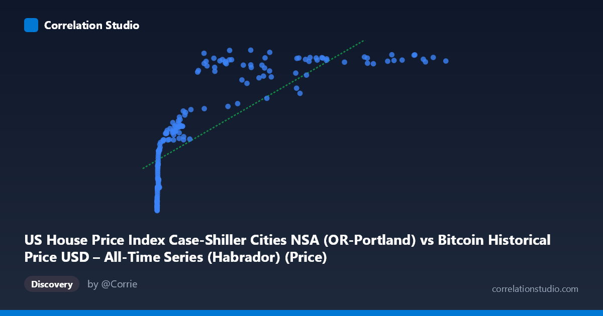
US House Price Index Case-Shiller Cities NSA (OR-Portland) vs Bitcoin Historical Price USD – All-Time Series (Habrador) (Price)
- Pearson correlation (r)
- 0.7811
- Spearman correlation
- 0.9568
- p-value
- 0
- Sample size (n)
- 189
- 95% confidence interval
- 0.7185 to 0.8312
- Granger causality
- None
- Granger optimal lag
- 9
- Time coverage
- 2010-08-01 to 2026-04-01
- Recomputed on refreshed data
- 2026-10-20 (r was 0.7763)
AI analysis
Analysis: Bitcoin Price vs. Portland Case-Shiller Home Price Index
1. What the Visualization Reveals
The scatterplot displays a strongly non-linear, saturating relationship between Bitcoin's USD price (X-axis, spanning nearly 6 orders of magnitude from $0.06 to $118,670) and the Portland Case-Shiller Home Price Index (Y-axis, ranging 129–342). Rather than a straight-line trend, the data shows a classic logarithmic curve: Y rises steeply as X moves from near-zero to a few thousand dollars, then flattens dramatically once Bitcoin exceeds ~$20,000–30,000, with the index plateauing in the 320–340 range even as Bitcoin pushes past $100,000.
2. Strength, Direction, and Statistical Meaning
The linear Pearson correlation (r = 0.776, R² = 0.603) indicates a strong positive linear relationship on its face, with 60% of Y's variance "explained" by X in a straight-line model. The 95% CI [0.712, 0.828] is tight and excludes zero, and the p-value of ~0 confirms this correlation is not due to chance — but this measures association, not causation or mechanism. Critically, the note that Spearman's ρ exceeds Pearson's r signals the true relationship is monotonic but curved (logarithmic/power-law), meaning the linear R² understates how tightly these variables actually track each other in rank-order terms. Most tellingly, Granger causality tests show no significant predictive direction in either direction (X→Y: p=0.545; Y→X: p=0.763). This is a crucial finding: despite the strong contemporaneous correlation, neither series helps forecast the other's future values — the relationship is not a temporal lead-lag one but likely reflects both variables independently trending upward over the same calendar period.
3. Notable Patterns and Outliers
The data clusters into two distinct regimes: (a) a low-X cluster (X < $1,000, mostly Bitcoin's 2010–2013 era) where Y ranges narrowly from ~129–220, and (b) a high-X cluster (X $20,000, 2020s era) where Y compresses into 260–340. The steep rise happens in the "middle" transition zone (roughly $1,000–$20,000). Some scatter/noise appears in the upper-middle range — e.g., points like (45092.81, 278.26) and (29111.52, 267.48) sit below the general trend, suggesting temporary housing dips or Bitcoin spikes that decouple the series. There are no extreme bivariate outliers; the residual scatter around the logarithmic curve is fairly consistent.
4. Confounding Factors and Caveats
This is almost certainly a spurious or confounded correlation driven by shared time trends, not a causal economic link. Both Bitcoin price and the Portland housing index have risen substantially since 2010–2011 due to entirely different macro drivers (crypto adoption/speculation vs. housing market fundamentals, low interest rates, migration to Portland, general inflation). Since both are non-stationary time series trending upward over the same 15+ year window, any two such series will show artificially inflated correlation — a well-known pitfall in time-series analysis. The lack of Granger causality reinforces that this is coincidental co-trending rather than a functional relationship. Additionally, comparing a global, 24/7 speculative asset to a single-city regional housing index is a mismatched pairing with no clear economic channel connecting them.
5. Actionable Insights
- Do not use this correlation for forecasting or trading strategies — the absence of Granger causality confirms neither series predicts the other. - Detrend or difference both series (e.g., use % monthly returns instead of levels) and re-run correlation; this will likely reveal the "true" relationship is much weaker, exposing the current r=0.78 as a trend artifact. - Fit a log(X) or power-law model instead of linear regression, given the Spearman/Pearson discrepancy — this should meaningfully improve model fit and better represent the saturating shape. - Treat this as a case study in spurious correlation for educational purposes rather than an actionable economic relationship; a more meaningful comparison would pair Bitcoin against variables with plausible causal links (e.g., risk-asset indices, USD liquidity measures, or interest rate policy).
X dataset: Bitcoin Historical Price USD – All-Time Series (Habrador)
Y dataset: US House Price Index Case-Shiller Cities NSA
Part of experiment: Bitcoin - Bitcoin Historical Price USD – All-Time Series (Habrador) vs US House Price Index Case-Shiller Cities NSA