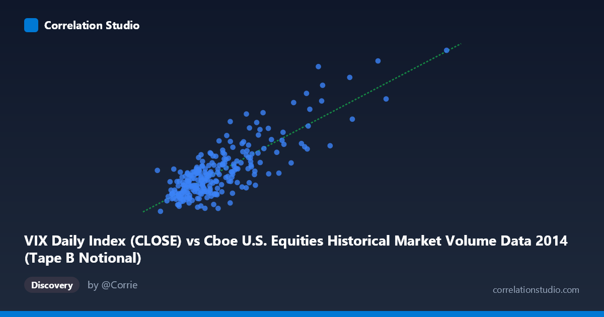
VIX Daily Index (CLOSE) vs Cboe U.S. Equities Historical Market Volume Data 2014 (Tape B Notional)

Pearson correlation (r): 0.8201
Spearman correlation: 0.7052
p-value: 0
Sample size (n): 252
95% confidence interval: 0.7751 to 0.8569
Granger causality: None
Granger optimal lag: 1

AI analysis

Scatterplot Analysis: VIX Daily Index vs. Tape B Notional Volume (2014)

Relationship Overview

The scatterplot reveals a positive, moderately strong linear relationship between the VIX Daily Index (Close) and Cboe U.S. Equities Tape B Notional trading volume across 252 trading days in 2014. As the VIX rises — indicating greater market fear and uncertainty — Tape B notional volume tends to increase correspondingly. This is conceptually intuitive: heightened volatility regimes typically drive elevated trading activity as institutional and retail participants reposition, hedge, or liquidate exposure. The linear regression equation (y = 1.39×10⁻⁹x + 8.07) captures this upward slope, though the wide X-axis range (roughly 2.1B to 13.0B) suggests substantial day-to-day variation in volume even at similar VIX levels.

Correlation Strength and Statistical Significance

The Pearson correlation of r = 0.8201 is statistically robust, with a p-value effectively at zero and a tight 95% confidence interval of [0.7751, 0.8569], leaving little doubt that the association is real and not a sampling artifact across the n = 252 paired observations. The R² of 0.6726 means approximately 67.3% of the variance in Tape B notional volume is explained by VIX levels — a meaningfully high figure for financial market data, though it equally implies that roughly one-third of volume variation remains unexplained by volatility alone. Despite this strong contemporaneous correlation, Granger causality tests find no significant temporal predictive direction in either direction (X→Y: F = 0.51, p = 0.48; Y→X: F = 0.02, p = 0.88). This is a critical nuance: VIX and Tape B volume move together, but neither reliably leads the other at a one-period lag, suggesting the relationship is largely coincident rather than predictive.

Notable Patterns, Clusters, and Outliers

Several structural features stand out in the data. The bulk of observations cluster densely in the lower-left region — VIX values roughly between 10 and 16 and notional volumes between 2.5B and 5.5B — reflecting the extended low-volatility environment that characterized much of early-to-mid 2014. However, a distinct upper-right cluster of high-leverage outliers is clearly visible, with points such as (10.4B, 25.20) and (9.4B, 23.57) representing the volatility spikes of October 2014 (the sharp equity selloff driven by Ebola fears and global growth concerns). These outlier observations exert significant influence on the regression slope and correlation coefficient, and the relationship may appear artificially tightened by these extreme joint observations. The spread around the regression line also appears to fan outward at higher VIX values — a possible sign of heteroscedasticity, where volume variability increases during stressed regimes.

Confounding Factors and Interpretive Caveats

Several important caveats apply. First, reverse causality is plausible in markets: surges in Tape B volume could themselves contribute to intraday volatility signals that feed into the VIX calculation, creating a reflexive feedback loop that inflates the observed correlation without implying a clean directional mechanism. Second, both variables may be jointly driven by unobserved macro events — geopolitical shocks, Federal Reserve communications, or earnings seasons — making this a classic case of omitted variable bias masquerading as a direct relationship. Third, the dataset covers only one calendar year (2014), a period notable for its unusual combination of low-volatility baseline and discrete spike events; the correlation structure may not generalize to other market regimes (e.g., 2008, 2020). Finally, Tape B specifically covers NYSE American and regional exchange listings, which may respond differently to volatility than broader market volume metrics.

Actionable Insights and Further Investigation

Practitioners and researchers should consider several follow-up directions. Given that Granger causality is absent at lag 1, testing longer lags (2–5 periods) or using intraday data may uncover lead-lag dynamics not visible at the daily frequency. It would be valuable to decompose the analysis by volatility regime — separating low-VIX (sub-15) from high-VIX (above-20) periods — to test whether the linear relationship holds symmetrically or whether the upper-right cluster is driving the bulk of explanatory power. Adding control variables such as S&P 500 returns, bid-ask spreads, or macroeconomic announcement indicators could help isolate the true marginal effect of volatility on volume. Finally, replicating this analysis across multiple years (particularly stress years like 2018 or 2020) would clarify whether the r = 0.82 figure is a stable structural feature of U.S. equity microstructure or an artifact of 2014's specific volatility profile.

X dataset: Cboe U.S. Equities Historical Market Volume Data 2014

Y dataset: VIX Daily Index

Part of experiment: Daily - Cboe U.S. Equities Historical Market Volume Data 2014 vs VIX Daily Index