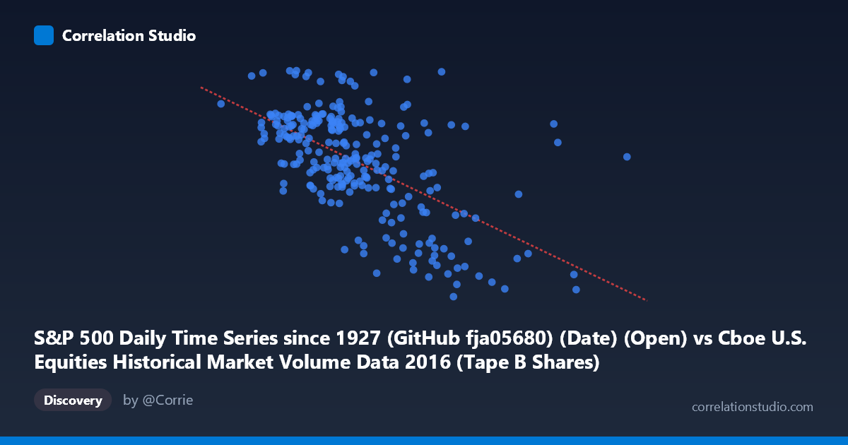
S&P 500 Daily Time Series since 1927 (GitHub fja05680) (Date) (Open) vs Cboe U.S. Equities Historical Market Volume Data 2016 (Tape B Shares)
- Pearson correlation (r)
- -0.5906
- Spearman correlation
- -0.568
- p-value
- 0
- Sample size (n)
- 252
- 95% confidence interval
- -0.6656 to -0.5038
- Granger causality
- None
- Granger optimal lag
- 1
AI analysis
Scatterplot Analysis: S&P 500 Open Price vs. Cboe Tape B Share Volume (2016)
Relationship Overview The scatterplot reveals a moderate negative relationship between the S&P 500 daily open price (X-axis) and Cboe Tape B share volume (Y-axis) across 252 trading days in 2016. As the S&P 500 open price increases throughout the year, Tape B share volume tends to decline — a pattern consistent with the well-documented inverse relationship between rising equity prices and trading volume during sustained bull market periods. The linear regression equation (y = −1.97×10⁻⁶x + 2305.43) confirms this downward slope, suggesting that for every ~500,000-point increase in the S&P 500 open, Tape B volume decreases by roughly 1 share unit on the Tape B scale used here.
Correlation Strength and Statistical Significance The Pearson correlation of r = −0.5906 indicates a moderate-to-strong negative association, and with r² = 0.3488, approximately 34.9% of the variance in Tape B volume is explained by the S&P 500 open price — meaningful but leaving roughly 65% attributable to other factors. The 95% confidence interval of [−0.6656, −0.5038] is entirely negative and relatively tight, reflecting strong confidence in the direction of the relationship. With a p-value effectively at zero across an N of 3,622 (population) and n of 252 (sample), the result is highly statistically significant and unlikely to be a chance finding. However, the Granger causality tests yield no significant predictive direction in either direction (X→Y: F=0.947, p=0.331; Y→X: F=0.820, p=0.366), meaning that despite the strong contemporaneous correlation, neither variable reliably predicts the other one period ahead. This is a critical distinction: correlation exists, but temporal forecasting power does not.
Notable Patterns, Clusters, and Outliers The data cloud shows a discernible but noisy downward sweep from the lower-left (lower prices, higher volume) to the upper-right (higher prices, lower volume). Several notable features stand out. A cluster of points in the 85M–115M price range with volume around 2,050–2,200 forms the dense core, representing the bulk of mid-year trading days. There are visible high-volume outliers at lower price levels — notably a point near (78.9M, 2,270) which represents the highest Tape B volume in the dataset, likely tied to an early January high-volatility session. Conversely, low-volume outliers at high price levels (e.g., ~170M open, ~1,861 volume) likely correspond to late-year sessions when the S&P 500 surged post-election but volume concentrated elsewhere. The scatter also appears to widen slightly at intermediate price levels, hinting at mild heteroscedasticity.
Confounding Factors and Caveats Several confounds warrant caution. First, time is a latent driver of both variables simultaneously: the S&P 500 trended upward throughout 2016, while volume patterns evolved seasonally and around specific events (Brexit, U.S. election), meaning the correlation may partly reflect shared time-trends rather than a direct economic linkage. Second, Tape B specifically covers NYSE American (AMEX) and regional exchange listings, which may respond to different investor segments than the broad S&P 500 index, making a mechanistic causal story harder to construct. Third, volume is measured in shares, not notional value, so shifts in stock price levels within Tape B listings could independently affect share count. Finally, the absence of Granger causality at lag-1 suggests this correlation is largely contemporaneous and structural, not a leading/lagging trading signal.
Actionable Insights and Further Investigation Practitioners should avoid using this correlation as a tactical trading signal, given the failed Granger causality tests. However, the relationship is useful for regime characterization: high Tape B volume days clustering at lower S&P 500 levels may serve as a volatility or stress indicator worth monitoring. Further investigation should include: (1) decomposing the time trend via detrended or first-differenced analysis to isolate genuine volume-price dynamics from shared drift; (2) testing longer Granger lags beyond 1 period, as market microstructure effects may operate over 2–5 day horizons; (3) examining whether VIX or realized volatility mediates this relationship, since fear-driven volume spikes at lower price levels would explain the pattern mechanically; and (4) comparing Tape A and Tape C volumes against the same price series to assess whether this inverse pattern is exchange-specific or market-wide.
X dataset: Cboe U.S. Equities Historical Market Volume Data 2016
Y dataset: S&P 500 Daily Time Series since 1927 (GitHub fja05680) (Date)
Part of experiment: Daily - Cboe U.S. Equities Historical Market Volume Data 2016 vs S&P 500 Daily Time Series since 1927 (GitHub fja05680) (Date)