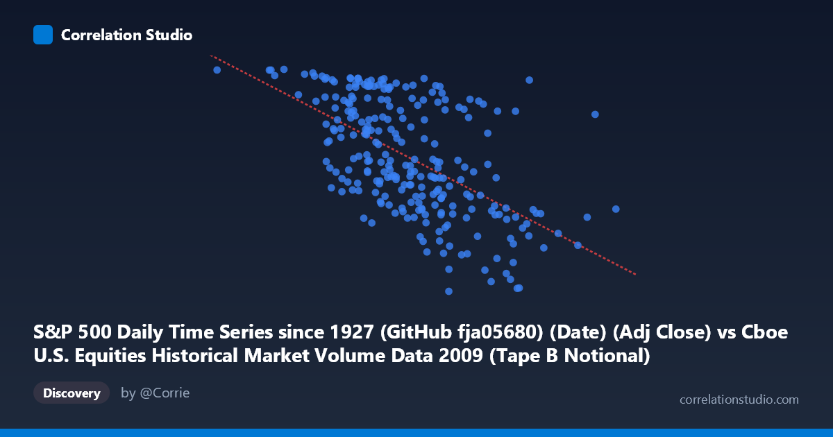
S&P 500 Daily Time Series since 1927 (GitHub fja05680) (Date) (Adj Close) vs Cboe U.S. Equities Historical Market Volume Data 2009 (Tape B Notional)

Pearson correlation (r): -0.5785
Spearman correlation: -0.5915
p-value: 0
Sample size (n): 252
95% confidence interval: -0.6552 to -0.49
Granger causality: Bidirectional
Granger optimal lag: 10

AI analysis

Analysis: S&P 500 Adjusted Close vs. Cboe Tape B Notional Volume (2009)

Relationship Overview The scatterplot reveals a moderate negative relationship between the S&P 500's adjusted closing price (X-axis, expressed as a Unix timestamp proxy for date) and Cboe Tape B notional trading volume (Y-axis). As the year 2009 progresses — with X values representing dates from January through December — Tape B notional volume generally declines, tracing an arc consistent with the dramatic market recovery of 2009. Early in the year, when the S&P 500 was near its crisis lows, notional volumes were elevated; as prices recovered through mid-to-late 2009, volume activity on Tape B contracted. This pattern is economically intuitive: panic-driven and distressed selling in early 2009 generated enormous notional turnover, which subsided as markets stabilized.

Correlation Strength and Statistical Significance The Pearson correlation of r = −0.578 indicates a moderate-to-strong negative association, with r² = 0.335, meaning approximately 33.5% of the variance in Tape B notional volume is explained by the temporal progression of S&P 500 prices alone. While statistically unambiguous (p ≈ 0, N = 3,232), the 95% confidence interval of [−0.655, −0.490] confirms the effect is meaningfully negative but leaves substantial unexplained variance — roughly 66.5% of Tape B notional fluctuation is driven by factors outside this simple linear relationship. The bidirectional Granger causality result (X→Y: F = 1.913, p = 0.045; Y→X: F = 1.878, p = 0.049) is notable: both series carry weak but statistically marginal predictive information about each other at a 10-period lag. However, these F-statistics are only marginally significant, and the feedback loop is better interpreted as a shared response to market conditions rather than true economic causation in either direction.

Notable Patterns, Clusters, and Outliers Several structural features are visible in the sample points. There is a high-volume cluster at low X values (early 2009 timestamps, e.g., X ≈ 1.32–2.43 billion range with Y values near 1,100–1,127), corresponding to the market bottom period around February–March 2009. Conversely, high X values (late 2009, X 7.5 billion) consistently show lower Y values (Y ≈ 683–770), consistent with reduced volatility-driven volume as the market recovered. The data also shows considerable vertical scatter at mid-range X values (X ≈ 4.5–6.5 billion), suggesting high day-to-day volume variability during the recovery phase. A few apparent outliers — such as the point near (7,526,902,255; 683) representing unusually low notional volume in late 2009 — may reflect holiday-shortened sessions or specific market events.

Confounding Factors and Caveats Several important caveats apply. First, X is fundamentally a time variable (Unix timestamp), meaning this correlation largely captures a temporal trend rather than a direct price-volume mechanism. The negative relationship may simply reflect that both variables are co-evolving with the broader 2009 recovery narrative. Second, Tape B specifically covers NYSE American (AMEX) and regional exchange stocks, which may have sector-specific dynamics (e.g., small-cap or ETF concentration) not representative of broader market volume. Third, the linear regression model (y = −5.11×10⁻⁸x + 1,217.38) imposes a linear structure on what appears to be a potentially non-linear or regime-dependent relationship — the scatter at mid-range X values suggests heteroscedasticity. Finally, volatility (VIX), institutional rebalancing flows, and specific policy events (e.g., stress test announcements in May 2009) are likely unmeasured confounders driving both price and volume simultaneously.

Actionable Insights and Further Investigation Practitioners should not interpret the Granger causality as tradeable signal given the marginal p-values and the 10-period lag structure, which may be spurious in a single-year dataset. More productive next steps would include: (1) decomposing the time trend by detrending both series and re-examining the residual correlation to isolate true price-volume dynamics from secular 2009 recovery effects; (2) introducing VIX or realized volatility as a covariate to test whether it absorbs the correlation; (3) comparing Tape B to Tape A and Tape C notional volumes to assess whether this pattern is exchange-specific or market-wide; and (4) extending the analysis across multiple years (2007–2012) to determine whether the negative price-volume relationship is a structural feature or an artifact of the crisis-recovery cycle. The bidirectional Granger result also warrants testing with VAR models incorporating additional control variables before drawing any predictive conclusions.

X dataset: Cboe U.S. Equities Historical Market Volume Data 2009

Y dataset: S&P 500 Daily Time Series since 1927 (GitHub fja05680) (Date)

Part of experiment: Daily - Cboe U.S. Equities Historical Market Volume Data 2009 vs S&P 500 Daily Time Series since 1927 (GitHub fja05680) (Date)