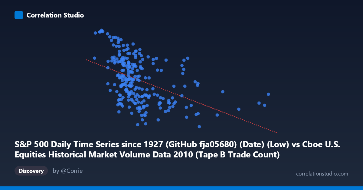
S&P 500 Daily Time Series since 1927 (GitHub fja05680) (Date) (Low) vs Cboe U.S. Equities Historical Market Volume Data 2010 (Tape B Trade Count)
- Pearson correlation (r)
- -0.4565
- Spearman correlation
- -0.5112
- p-value
- 0
- Sample size (n)
- 252
- 95% confidence interval
- -0.5491 to -0.3529
- Granger causality
- None
- Granger optimal lag
- 1
AI analysis
Analysis: S&P 500 Daily Low vs. Cboe Tape B Trade Count (2010)
Relationship Overview The scatterplot reveals a moderate negative relationship between the S&P 500 daily low price (X-axis) and the Cboe Tape B trade count (Y-axis) across 2010. As the index's daily low increases — meaning the market is trading at higher price levels — the number of Tape B trades tends to decrease. The linear regression equation (y = −0.000208x + 1,194.31) quantifies this inverse slope, suggesting that for every 100,000-point increase in the daily low, trade count drops by roughly 20–21 units. Visually, this manifests as a downward-sloping cloud of points, though with considerable scatter around the trend line, indicating the relationship is real but far from deterministic.
Correlation Strength and Statistical Significance The Pearson correlation of r = −0.457 represents a moderate negative association, and the R² of 0.208 tells the more grounded story: only about 20.8% of the variance in Tape B trade counts is explained by variation in the S&P 500 daily low. That leaves nearly 80% of the variance unexplained by this variable alone, underscoring that many other forces drive trading activity. The relationship is nonetheless highly statistically significant (p = 2.22×10⁻¹⁴), making it extremely unlikely to be a chance artifact given the sample of 252 paired observations. The 95% confidence interval for r of [−0.549, −0.353] is reassuringly tight and entirely negative, confirming the direction of the effect is reliable. However, Granger causality tests find no significant temporal predictive direction in either direction (X→Y: F = 2.17, p = 0.142; Y→X: F = 3.23, p = 0.074), meaning that knowing yesterday's S&P 500 low does not statistically improve next-day forecasts of Tape B trade counts beyond baseline, and vice versa. This is a crucial caveat: the correlation is contemporaneous, not predictively causal.
Notable Patterns, Clusters, and Outliers Several structural features stand out in the data. There is a dense cluster of points in the lower X range (roughly 95,000–350,000), where trade counts span a wide range from ~1,040 to ~1,260, suggesting high variability in trading activity during periods of lower index prices (likely earlier in 2010 when the market had not yet fully recovered). At higher X values — above 500,000 — points are sparser and tend to cluster in the lower Y range (1,040–1,130), consistent with the negative trend. A few notable outliers deserve attention: the point near (918,660, 1,094) sits far to the right as the maximum X value yet has only a mid-range trade count, and points near (120,757, 1,254) and (134,700, 1,255) anchor the upper-left corner with very high trade counts at low price levels. These extremes disproportionately influence the regression slope and correlation coefficient.
Confounding Factors and Interpretive Caveats The negative correlation almost certainly reflects a temporal confound: 2010 was a recovery year for U.S. equities, with the S&P 500 trending upward over the calendar year. As prices rose throughout the year, it is plausible that retail and high-frequency trading participation — which heavily influences Tape B (smaller-cap/regional exchange) trade counts — evolved differently from index price dynamics. What appears to be a price-activity relationship may largely be two time series trending in opposite directions over the same period. Additionally, Tape B trade counts are influenced by exchange-specific factors such as routing rules, fee structures, and competitive dynamics among venues, none of which are captured by S&P 500 pricing. The N = 3,302 population size versus n = 252 sample also warrants noting — while the sample is reasonably representative, the inference is drawn from one calendar year only.
Actionable Insights and Further Investigation Despite the caveats, the findings point to several productive next steps. Detrending both series (e.g., using first-differences or residuals from a time trend) would isolate whether a genuine contemporaneous relationship persists beyond the shared upward/downward drift of 2010. Extending the analysis across multiple years would test whether this negative correlation is a structural feature of the market or an artifact of 2010's specific recovery trajectory. It would also be valuable to include other Tape classifications (A and C) to determine whether the effect is concentrated in Tape B or represents broader market behavior. Finally, since Granger causality was borderline for Y→X (p = 0.074), testing at slightly longer lags or with higher-frequency intraday data may reveal whether elevated Tape B activity subtly precedes index price movements — a potentially actionable signal for market microstructure research.
X dataset: Cboe U.S. Equities Historical Market Volume Data 2010
Y dataset: S&P 500 Daily Time Series since 1927 (GitHub fja05680) (Date)
Part of experiment: Daily - Cboe U.S. Equities Historical Market Volume Data 2010 vs S&P 500 Daily Time Series since 1927 (GitHub fja05680) (Date)