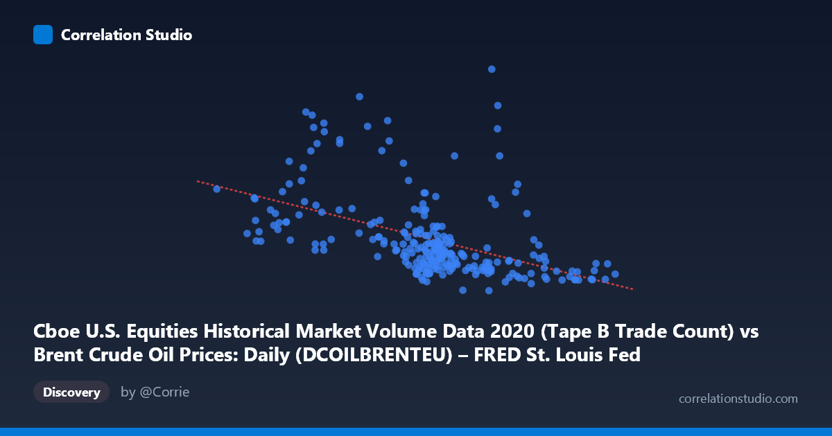
Cboe U.S. Equities Historical Market Volume Data 2020 (Tape B Trade Count) vs Brent Crude Oil Prices: Daily (DCOILBRENTEU) – FRED St. Louis Fed (DCOILBRENTEU)
- Pearson correlation (r)
- -0.4749
- Spearman correlation
- -0.5921
- p-value
- 0
- Sample size (n)
- 250
- 95% confidence interval
- -0.5656 to -0.3728
- Granger causality
- None
- Granger optimal lag
- 10
AI analysis
Scatterplot Analysis: Cboe Tape B Trade Count vs. Brent Crude Oil Price (2020)
1. Overall Relationship Pattern
The scatterplot reveals a moderate negative relationship between Cboe U.S. Equities Tape B trade count and Brent Crude Oil prices across 2020. As equity trade counts increase, crude oil prices tend to decline, and vice versa. However, the scatter is substantial — data points are widely dispersed around the regression line (y = -7667.27x + 737,033), indicating that the linear trend captures only a portion of the underlying dynamics. The distribution is notably heteroscedastic, with considerably wider Y-axis spread at lower X values (roughly below 30), suggesting that when equity trade volumes are low, oil price outcomes become far more variable and unpredictable.
2. Correlation Strength, Direction, and Temporal Causality
The Pearson r of -0.4749 reflects a moderate negative correlation, statistically highly significant (p = 1.776E-15) given the large population size of N = 4,254. Yet practical significance deserves careful framing: r² = 0.2255 means only ~22.6% of the variance in Brent crude prices is explained by Tape B trade count, leaving roughly 77% attributable to other factors. The 95% confidence interval of [-0.5656, -0.3728] is meaningfully narrow, confirming that the negative direction is robust and not a sampling artifact, but also confirming the relationship is firmly in "moderate" territory — it would be incorrect to characterize this as a strong predictive link. Critically, the Granger causality tests find no significant temporal predictive direction in either direction (X→Y: F = 0.4093, p = 0.9414; Y→X: F = 0.2605, p = 0.9887 at optimal lag 10), meaning that past values of trade count do not reliably forecast future oil prices and vice versa. This is a crucial caveat: the observed correlation reflects a contemporaneous co-movement, not a leading indicator relationship in either direction.
3. Notable Patterns, Clusters, and Outliers
Several features stand out visually:
- High-variance cluster at low X values (X < 30): A small but influential cluster of points in this range spans Y values from approximately 360,000 to over 1,200,000 — an enormous spread. These likely correspond to March–April 2020 pandemic shock periods, when equity volumes were unusual and oil prices were simultaneously collapsing due to the Saudi-Russia price war and demand destruction. This cluster heavily influences the regression slope. - Dense central cluster (X ≈ 38–50): The bulk of observations cluster here with Y values concentrated between ~220,000 and ~620,000, reflecting more "normal" 2020 trading conditions during mid-year recovery. The relationship here is weaker and noisier. - Notable outlier at approximately (35.33, 977,851): This point sits far above the regression line and may represent a specific date with anomalous volume or price behavior worth individual investigation. - Right-tail compression (X 55): At higher trade counts, oil prices appear consistently low and less variable, consistent with a floor-like compression — suggesting a possible non-linear, possibly logarithmic or power-law relationship. The note that Spearman ρ exceeds Pearson r formally supports this interpretation, meaning a non-linear model (polynomial or logarithmic) would better capture the true functional form.
4. Confounding Factors and Interpretive Caveats
Several confounders complicate straightforward interpretation:
- 2020 was a structurally exceptional year. The COVID-19 pandemic, the OPEC+ price war (March 2020), and unprecedented monetary/fiscal interventions created regime shifts that violate stationarity assumptions underlying standard correlation analysis. The negative correlation may largely reflect these extraordinary co-shocks rather than a stable structural relationship. - Simultaneity and common-cause bias: Both equity trading volume and oil prices respond to the same macroeconomic news shocks (e.g., lockdown announcements, OPEC meetings, Fed decisions). Their correlation may be a spurious artifact of shared third-variable exposure rather than any direct linkage. - Tape B specificity: Tape B covers regional exchanges (NYSE American, NYSE Arca, etc.), not the full equity market. Using total market volume or S&P 500 futures volume might yield different results and better represent the macroeconomic signal. - Temporal aggregation: Daily data mixes intraday patterns and calendar effects. The Granger lag of 10 periods may span two full trading weeks, and the lack of causality at this horizon doesn't preclude very short-term (intraday or 1–2 day) relationships not testable with daily data. - The axes appear swapped in labeling (the dataset descriptions suggest the column assignments may be reversed from what's described), which should be verified before drawing operational conclusions.
5. Actionable Insights and Further Investigation
- Fit a non-linear model (logarithmic or piecewise linear with a structural break around March 2020) to better capture the functional form suggested by the Spearman-Pearson discrepancy; this could meaningfully improve explained variance beyond 22.6%. - Segment the analysis by market regime: Separate the pandemic shock period (January–May 2020) from the recovery period (June–December 2020) and run correlations independently. The overall correlation likely masks two very different sub-period relationships. - Test shorter Granger lags (1–5 days): The optimal 10-period lag may be too long to detect intraday or next-day information transmission; testing at lags 1–5 with higher-frequency data could reveal whether equity market stress signals oil price moves in near-real-time. - Incorporate VIX or credit spreads as covariates in a multivariate regression to test whether the Tape B–oil relationship survives after controlling for broader market fear/risk-off dynamics, which likely drive both variables simultaneously. - Investigate the outlier cluster (low X, high Y) by mapping specific dates — these are likely March 2020 observations that disproportionately drive the regression slope and should be tested for undue leverage using Cook's distance or hat-matrix diagnostics.
X dataset: Brent Crude Oil Prices: Daily (DCOILBRENTEU) – FRED St. Louis Fed
Y dataset: Cboe U.S. Equities Historical Market Volume Data 2020
Part of experiment: Daily - Brent Crude Oil Prices: Daily (DCOILBRENTEU) – FRED St. Louis Fed vs Cboe U.S. Equities Historical Market Volume Data 2020