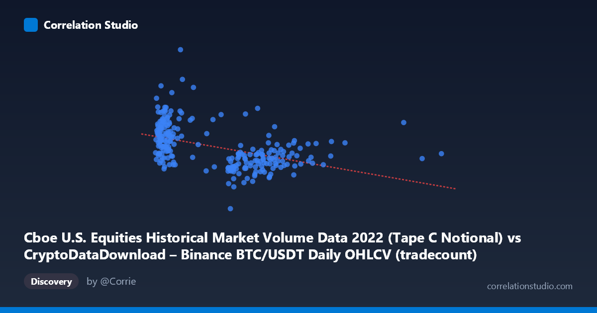
Cboe U.S. Equities Historical Market Volume Data 2022 (Tape C Notional) vs CryptoDataDownload – Binance BTC/USDT Daily OHLCV (tradecount)
- Pearson correlation (r)
- -0.458
- Spearman correlation
- -0.4976
- p-value
- 0
- Sample size (n)
- 251
- 95% confidence interval
- -0.5506 to -0.3543
- Granger causality
- None
- Granger optimal lag
- 10
AI analysis
Analysis: Cboe Equities Volume vs. BTC/USDT Trade Count (2022)
1. Overall Relationship
The scatterplot shows a moderate negative, non-linear relationship between the two variables. At low X values (roughly 800,000–2,500,000), Y is highly dispersed, ranging from ~10 billion to over 22 billion, indicating substantial variance in trade count that is not explained by equity volume at this range. As X increases beyond ~3,000,000, the Y values compress into a narrower, lower band (roughly 9–13 billion), producing the visual impression of a downward-sloping cloud. This pattern looks less like a single linear relationship and more like a "fan" or "wedge" shape — heteroscedastic, with variance in Y shrinking as X grows.
2. Strength, Direction, and Statistical Confidence
The correlation coefficient (r = -0.458) indicates a moderate negative linear association, with the linear model explaining only 21.0% of the variance in tradecount (R² = 0.2098). This means nearly 80% of the variation in Y is driven by factors outside this X variable — the relationship, while statistically real, has limited practical predictive power on its own. The 95% CI [-0.551, -0.354] is reasonably tight and excludes zero, and the p-value (2.02E-14) confirms this correlation is highly unlikely to be due to chance in this sample. However, statistical significance should not be conflated with strength or causal relevance — the confidence interval still spans a fairly wide range of "moderate" correlation strengths, so precision about the exact effect size is limited.
Critically, the Granger causality tests found no significant predictive direction in either direction (X→Y: p=0.109; Y→X: p=0.443) at the optimal lag of 10 periods. This suggests that despite the contemporaneous correlation, neither series reliably predicts future values of the other in a time-series sense. This is an important distinction: the relationship may be driven by both series independently trending against a shared external factor (e.g., macro market conditions, seasonality, or volatility regimes in 2022) rather than one causing the other.
3. Notable Patterns and Outliers
Several high-leverage points stand out: values like (1,065,054, 21.19B), (2,092,561, 22.09B), and (1,248,246, 17.75B) sit well above the general trend and pull the regression line's slope. These appear at low X values, suggesting occasional spikes in BTC tradecount unrelated to equity volume — possibly driven by crypto-specific volatility events (e.g., news-driven trading days) rather than equity market activity. The clustering of points at X < 2,000,000 with high Y variance versus the tighter cluster at X 4,000,000 with lower, more stable Y values suggests two different volume regimes rather than one continuous linear process — potentially corresponding to different periods or volatility states in 2022 (e.g., early-year vs. later-year market conditions).
4. Confounding Factors and Caveats
Both series are time-ordered financial/market datasets from 2022, a year marked by macro-driven volatility (rate hikes, crypto crashes like Terra/Luna and FTX). Both BTC tradecount and equity volume could be responding to the same macro volatility shocks independently, creating spurious correlation without direct causal linkage — consistent with the null Granger result. Additionally, comparing a crypto exchange's tradecount to Cboe equity notional volume conflates different market structures, asset classes, and participant bases; any correlation may reflect broad "risk-on/risk-off" sentiment rather than a mechanistic relationship. The non-constant variance (heteroscedasticity) also violates a core assumption of linear regression, meaning the R² and regression coefficients likely understate the complexity of the true relationship.
5. Suggestions for Further Investigation
Given the heteroscedasticity, consider a log transformation of one or both variables, or a rank-based (Spearman) correlation to check if the relationship is more monotonic than linear. Segment the data by time period (e.g., pre/post major 2022 crypto events) to test whether the relationship is regime-dependent rather than stable across the year. Since Granger causality is insignificant, explore whether both series are jointly driven by a third variable (e.g., VIX, overall market volatility index, or a crypto volatility index) using multivariate models. Finally, given the outliers with low equity volume but extreme BTC tradecount, a closer date-level investigation of those specific days could reveal event-driven anomalies worth excluding or modeling separately.
X dataset: CryptoDataDownload – Binance BTC/USDT Daily OHLCV
Y dataset: Cboe U.S. Equities Historical Market Volume Data 2022
Part of experiment: Bitcoin - CryptoDataDownload – Binance BTC/USDT Daily OHLCV vs Cboe U.S. Equities Historical Market Volume Data 2022