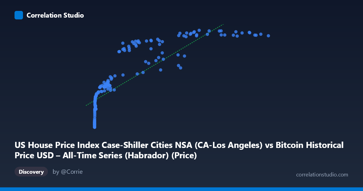
US House Price Index Case-Shiller Cities NSA (CA-Los Angeles) vs Bitcoin Historical Price USD – All-Time Series (Habrador) (Price)
- Pearson correlation (r)
- 0.8295
- Spearman correlation
- 0.9705
- p-value
- 0
- Sample size (n)
- 187
- 95% confidence interval
- 0.7787 to 0.8695
- Granger causality
- None
- Granger optimal lag
- 9
AI analysis
Analysis: Bitcoin Price vs. Case-Shiller LA Home Price Index
1. What the Visualization Reveals
The scatterplot shows a strong positive association between Bitcoin's historical USD price (X-axis) and the Case-Shiller Los Angeles home price index (Y-axis). However, the relationship is clearly non-linear: at low Bitcoin prices (under ~$1,000), the home price index varies substantially (roughly 160–260) with a steep initial rise, while at high Bitcoin prices (tens of thousands to $118,670), the index compresses into a narrower band (400–450). This creates a curved, logarithmic-like shape rather than a straight line — the index appears to respond to relative growth in Bitcoin price rather than absolute dollar increases.
2. Strength, Direction, and Uncertainty
The Pearson correlation (r = 0.83, R² = 0.688) indicates a strong positive linear relationship, with roughly 69% of variance in the housing index statistically explained by Bitcoin price under a linear model. The 95% CI [0.779, 0.870] is tight and the p-value is effectively 0, meaning this correlation is highly unlikely to be a sampling artifact within this dataset. That said, statistical significance here should not be confused with causal or mechanistic meaning — the note that Spearman's ρ exceeds Pearson's r confirms the relationship is monotonic but non-linear, so the linear R² likely understates the true strength of association once curvature is modeled properly (e.g., log-transforming X).
Critically, the Granger causality tests show no significant predictive direction in either direction (X→Y: p=0.766; Y→X: p=0.796) at the optimal lag of 9 periods. This means neither variable helps forecast the other's future values based on past values — despite the strong contemporaneous correlation, there is no evidence of a lead-lag temporal relationship. This is a classic signature of two variables driven by a shared external trend (e.g., time, monetary policy, inflation) rather than one causing the other.
3. Notable Patterns and Outliers
Several structural features stand out: - Compression at scale: Most high-value Bitcoin prices ($50,000+) map to a narrow home-price band (~410–451), suggesting diminishing marginal association — the housing index is not growing at the same rate as Bitcoin. - Early volatility: Very low Bitcoin prices (near $0–$100) still correspond to a fairly wide range of housing values (160–215), reflecting that housing was already appreciating independent of Bitcoin's early micro-fluctuations. - Plateau/dip anomalies: Some mid-range points break the trend (e.g., $58,724 → 339.43 and $45,092 → 333.24 sit well below neighboring points like $57,454 → 437.37), which likely correspond to a housing market correction (e.g., 2022 rate-hike slowdown) coinciding with Bitcoin price levels from a different market cycle — evidence that time, not Bitcoin price, is the real driver of housing moves.
4. Confounders and Caveats
This is very likely a spurious or common-trend correlation. Both series are heavily influenced by time itself — Bitcoin has undergone secular, multi-cycle appreciation since 2010, and the Case-Shiller LA index has appreciated steadily due to unrelated macroeconomic housing fundamentals (interest rates, wage growth, inventory shortages, migration patterns). Because both variables are strongly trending with time, any two upward-trending series will show high correlation without any causal linkage. Additionally: - Data are highly autocorrelated (monthly time series), violating the independence assumption behind standard p-value interpretation — the "true" effective sample size is much smaller than n=187. - Bitcoin's extreme right-skewed distribution (mean 20,037 vs. stdev 29,663) means a handful of high-price observations exert outsized leverage on the linear fit.
5. Actionable Recommendations
- Detrend or difference both series (e.g., use year-over-year % changes instead of levels) before assessing correlation — this is the standard fix for spurious trend-driven correlation in time series. - Log-transform Bitcoin price given its exponential growth pattern; refitting with log(X) will likely substantially improve model fit and better reflect the true (non-linear) relationship, consistent with the Spearman/Pearson divergence. - Treat this as a non-causal association for forecasting purposes — the null Granger result means Bitcoin price should not be used as a leading indicator for LA home prices (or vice versa) in any predictive model. - Consider adding a genuine macro confounder (e.g., M2 money supply, CPI, or mortgage rates) as a control variable to test whether the Bitcoin–housing correlation disappears once shared monetary/inflationary drivers are accounted for.
X dataset: Bitcoin Historical Price USD – All-Time Series (Habrador)
Y dataset: US House Price Index Case-Shiller Cities NSA
Part of experiment: Bitcoin - Bitcoin Historical Price USD – All-Time Series (Habrador) vs US House Price Index Case-Shiller Cities NSA