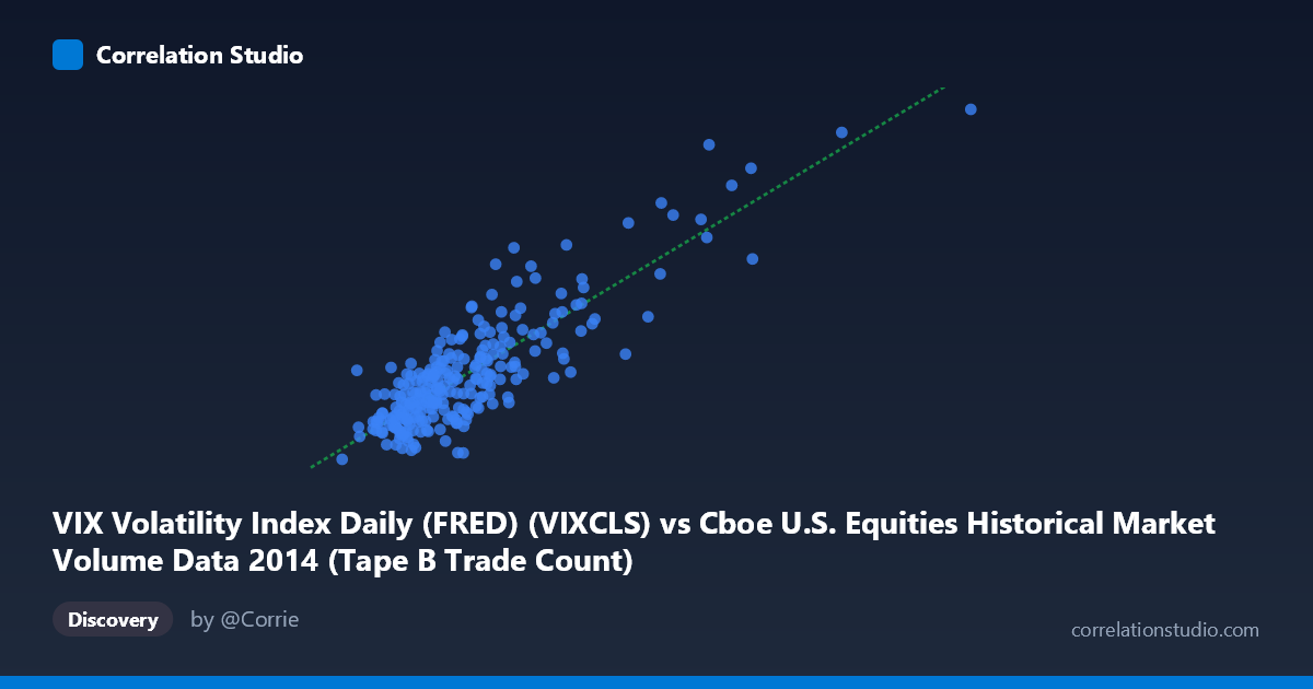
VIX Volatility Index Daily (FRED) (VIXCLS) vs Cboe U.S. Equities Historical Market Volume Data 2014 (Tape B Trade Count)
- Pearson correlation (r)
- 0.8566
- Spearman correlation
- 0.7577
- p-value
- 0
- Sample size (n)
- 252
- 95% confidence interval
- 0.8198 to 0.8863
- Granger causality
- None
- Granger optimal lag
- 1
AI analysis
Analysis: VIX Volatility Index vs. Tape B Trade Count (2014)
Relationship Overview The scatterplot reveals a strong positive relationship between the CBOE VIX Volatility Index and Tape B trade counts on U.S. equities exchanges throughout 2014. As market volatility rises (higher VIX), trading activity on Tape B venues increases substantially. The linear regression equation (y = 3.04×10⁻⁵x + 7.44) confirms this upward trend, suggesting that for every unit increase in VIX, Tape B trade counts rise by approximately 30,400 units. This is an intuitively sensible relationship — periods of market stress and uncertainty tend to drive elevated trading activity as investors reposition, hedge, or react to news events.
Correlation Strength and Statistical Significance The correlation is notably strong (r = 0.8566), with R² = 0.7337 indicating that approximately 73.4% of the variance in Tape B trade counts is explained by VIX levels alone — a remarkably high figure for financial market data. The 95% confidence interval [0.8198, 0.8863] is relatively narrow, reflecting high precision in the estimate, and the p-value of effectively zero confirms this relationship is not attributable to chance across the 252 paired observations. However, despite this strong contemporaneous correlation, the Granger causality tests reveal no significant predictive directionality in either direction (X→Y: F=0.5957, p=0.441; Y→X: F=0.0083, p=0.928). This is a critical nuance: VIX and Tape B volume move together, but neither meaningfully predicts the other's future values at a one-period lag. The relationship is essentially synchronous rather than predictive.
Patterns, Clusters, and Outliers The sample points reveal several notable structural features. The bulk of observations cluster in the lower-left region (VIX roughly 110,000–250,000; trade counts between 11–16), consistent with 2014's generally low-volatility environment. However, there are clear high-leverage outliers in the upper-right quadrant — notably points near (559,868, 25.20) and (478,251, 23.57) — which likely correspond to discrete market stress episodes such as the October 2014 volatility spike. These outliers appear to follow the linear trend rather than break from it, suggesting the relationship holds even during tail events. There is also a subtle hint of heteroscedasticity: variance in trade counts appears to increase at higher VIX levels, which may slightly inflate the linear R² and warrants further examination with robust regression methods.
Confounding Factors and Caveats Several important caveats apply. First, 2014 was a predominantly low-volatility year punctuated by brief spikes, meaning the correlation may be heavily influenced by a small number of extreme observations; removing the top 5–10% of VIX readings could substantially alter the relationship. Second, Tape B trade counts are influenced by many factors beyond volatility, including exchange fee schedules, algorithmic trading strategies, seasonal patterns, and structural market changes — all potential confounders. Third, the axis labels appear swapped in the dataset metadata (VIX is on X-axis per the chart but labeled as the Y-axis dataset source), which should be verified before drawing firm conclusions. Finally, the N=3,686 population size versus n=252 sample suggests this analysis covers a subset of available data, and results should be validated on the full population.
Actionable Insights and Further Investigation Practitioners should investigate whether the relationship holds across multiple years (2010–2023) to confirm structural stability, particularly through the COVID-19 volatility shock of 2020. Given the absence of Granger causality, trading strategies predicated on using VIX to predict next-day Tape B volume (or vice versa) are unlikely to be profitable — attention should shift to contemporaneous modeling rather than lagged prediction. It would also be valuable to decompose Tape B volume by trade size or participant type (retail vs. institutional) to understand which actors drive the VIX-volume nexus. Finally, applying a log transformation to both variables could address the apparent heteroscedasticity and potentially reveal whether the relationship is better characterized as a power-law rather than a linear one.
X dataset: Cboe U.S. Equities Historical Market Volume Data 2014
Y dataset: VIX Volatility Index Daily (FRED)
Part of experiment: Daily - Cboe U.S. Equities Historical Market Volume Data 2014 vs VIX Volatility Index Daily (FRED)