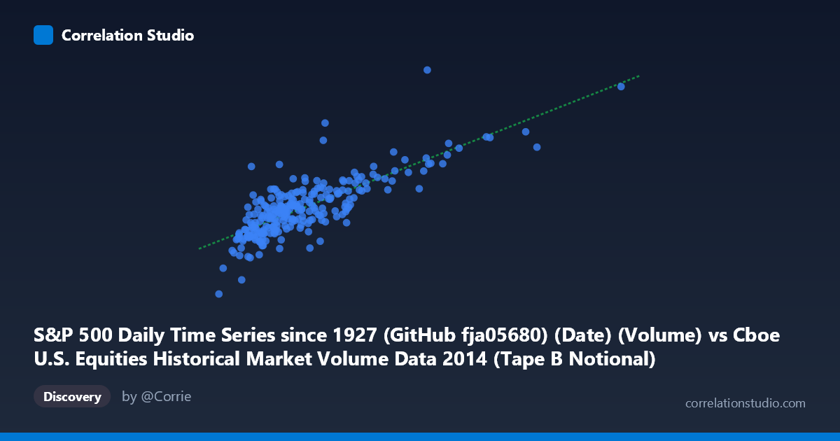
S&P 500 Daily Time Series since 1927 (GitHub fja05680) (Date) (Volume) vs Cboe U.S. Equities Historical Market Volume Data 2014 (Tape B Notional)
- Pearson correlation (r)
- 0.7916
- Spearman correlation
- 0.7456
- p-value
- 0
- Sample size (n)
- 252
- 95% confidence interval
- 0.7405 to 0.8336
- Granger causality
- None
- Granger optimal lag
- 10
AI analysis
Analysis: S&P 500 Trading Volume vs. Cboe Tape B Notional Value (2014)
Relationship Overview The scatterplot reveals a moderate-to-strong positive relationship between S&P 500 daily trading volume and Cboe Tape B notional value across 252 trading days in 2014. As overall market volume increases, the notional value transacted on Tape B (which covers NYSE American-listed securities) rises in a broadly linear fashion, consistent with the regression equation y = 0.327x + 1.92B. This makes intuitive sense: both metrics are expressions of market activity intensity, and days characterized by elevated participation tend to lift trading value across exchange tapes simultaneously. The relationship, while coherent, is not perfectly tight — there is visible scatter around the regression line, particularly at higher volume levels.
Correlation Strength and Statistical Framing The Pearson correlation of r = 0.7916 indicates a strong positive association, and the R² of 0.6266 tells us that approximately 62.7% of the variance in Tape B notional value is explained by overall S&P 500 volume — meaningful explanatory power, but leaving ~37% attributable to other factors. The 95% confidence interval [0.7405, 0.8336] is relatively narrow, reflecting the robustness of the estimate given n = 252 paired observations drawn from a population of N = 3,686, and the p-value of ~0 confirms this correlation is not a sampling artifact. However, the Granger causality results introduce an important caveat: neither variable significantly predicts the other temporally (X→Y: F = 1.08, p = 0.379; Y→X: F = 0.74, p = 0.683). This means the two series move together contemporaneously, but neither leads the other — the correlation is synchronous rather than predictive, even at the optimal lag of 10 periods.
Patterns, Clusters, and Outliers The bulk of observations cluster in the lower-left region, with X values between roughly 2.9B–5.5B and Y values between 2.5B–4.2B, suggesting most trading days in 2014 were relatively unremarkable in volume terms. Several prominent outliers appear in the upper-right quadrant — most notably points near X ≈ 10.4B (Y ≈ 5.07B) and X ≈ 9.4B (Y ≈ 4.96B) — likely corresponding to high-volatility events such as geopolitical shocks or Fed announcements during 2014. One point near (2.74B, 1.74B) sits notably low on both axes, possibly reflecting a holiday-shortened session. There is also a suggestion of mild heteroscedasticity: variance in Y appears to widen as X increases, hinting that the linear model may underfit high-volume regimes.
Confounding Factors and Caveats Several confounds complicate causal interpretation. First, both variables are proxies for the same underlying latent driver — aggregate investor activity — so their correlation may largely reflect shared exposure to market-wide sentiment, volatility (VIX spikes), or macro announcements rather than any structural link between the S&P 500 composite volume and Tape B specifically. Second, Tape B notional is also price-sensitive: a given number of shares traded generates higher notional on days when prices are elevated, introducing a price-level confound independent of volume. Third, the dataset is confined to a single calendar year (2014), a period of generally low volatility and unidirectional equity appreciation, which may compress the range of conditions and inflate the apparent correlation relative to a multi-year sample.
Actionable Insights and Further Investigation The synchronous but non-predictive nature of this relationship suggests that Tape B notional cannot be used as a leading indicator for broad market volume (or vice versa), limiting tactical utility. Further investigation should: (1) extend the time horizon across multiple market regimes (e.g., 2008, 2020) to test whether the correlation and R² are stable or regime-dependent; (2) decompose notional value into price and volume components to isolate whether the driver is share count or price-level effects; (3) test nonlinear models (e.g., log-log regression or spline fits) given the potential heteroscedasticity at high volumes; and (4) examine residuals around known market events in 2014 (Russia-Ukraine escalation, October correction) to determine whether structural breaks explain the outlier cluster, which could inform risk-monitoring frameworks for exchange-level liquidity.
X dataset: Cboe U.S. Equities Historical Market Volume Data 2014
Y dataset: S&P 500 Daily Time Series since 1927 (GitHub fja05680) (Date)
Part of experiment: Daily - Cboe U.S. Equities Historical Market Volume Data 2014 vs S&P 500 Daily Time Series since 1927 (GitHub fja05680) (Date)