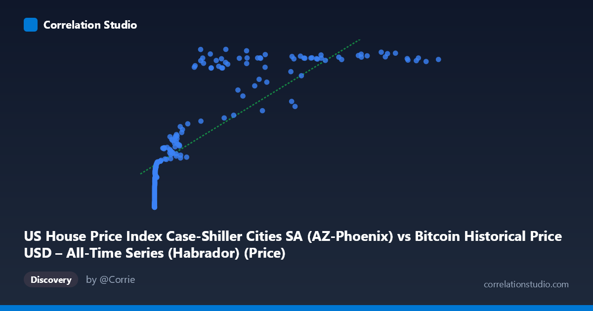
US House Price Index Case-Shiller Cities SA (AZ-Phoenix) vs Bitcoin Historical Price USD – All-Time Series (Habrador) (Price)
- Pearson correlation (r)
- 0.8214
- Spearman correlation
- 0.9563
- p-value
- 0
- Sample size (n)
- 191
- 95% confidence interval
- 0.7691 to 0.8628
- Granger causality
- None
- Granger optimal lag
- 9
- Time coverage
- 2010-08-01 to 2026-06-01
- Recomputed on refreshed data
- 2026-10-24 (r was 0.8174)
AI analysis
Analysis: Bitcoin Price vs. Phoenix Case-Shiller Home Price Index
1. What the Visualization Reveals
The scatterplot shows a strong positive association between Bitcoin's historical price and the Phoenix (AZ) Case-Shiller home price index, but the relationship is clearly non-linear. At low Bitcoin prices (under ~$1,000), the home price index climbs steeply from ~100 to ~190 despite tiny changes in X. Once Bitcoin exceeds roughly $20,000–30,000, the index compresses into a narrow band (~310–335), producing a curve that resembles a logarithmic or saturating function rather than a straight line. This is reinforced by the note that Spearman's ρ exceeds Pearson's r — the variables are monotonically related more consistently than linearly related.
2. Strength, Direction, and Uncertainty
The Pearson correlation (r = 0.813, r² = 0.661) indicates a strong positive linear relationship, with 66% of the variance in the home price index statistically explained by Bitcoin price under a linear model. The 95% CI [0.758, 0.857] is fairly tight and the p-value (~0) confirms this correlation is not due to chance in the sampled data. However, correlation here almost certainly reflects shared temporal trend rather than causal linkage: both series have risen over the 2010–2026 window, and the Granger causality tests explicitly show no predictive relationship in either direction (Bitcoin→Housing: p=0.72; Housing→Bitcoin: p=0.84, at 9 lags). This is a critical finding — despite the strong contemporaneous correlation, neither variable helps forecast the other's future values, undermining any causal or leading-indicator interpretation.
3. Notable Patterns and Outliers
Several structural features stand out: - Two-regime behavior: a rapid-rise phase (X < $1,000) and a plateau phase (X $20,000) where the housing index hugs a ceiling near 320–335 regardless of further Bitcoin appreciation (e.g., $27,983 → 325.10 vs. $118,670 → 323.93). - A visible dip/outlier cluster around X ≈ $29,000–58,000 where Y drops to 235–283 (e.g., 29,111.52 → 235.23; 45,092.81 → 246.30; 58,724.66 → 252.74) before rebounding to the 320s at similar or lower X values. This suggests a temporal loop — Bitcoin likely revisited similar price levels across different market cycles (2018 crash, 2021 peak, 2022 correction) while housing continued its own independent trajectory. - Compression at high X: the top ~40% of Bitcoin's range (X $60,000) maps to a very narrow Y range, contributing to the apparent flattening/saturation shape.
4. Confounding Factors and Caveats
This is a classic case of spurious correlation via mutual trend: both Bitcoin price and US housing indices have experienced long-term secular growth over the 2010–2026 period, driven by macro factors like low interest rates (2010s), pandemic-era stimulus, inflation, and speculative asset demand — not by any direct economic mechanism linking crypto prices to Phoenix home values. Time itself is the likely lurking variable. Additionally, pairing by row index/date rather than by matched timestamps could introduce alignment artifacts, and the sample skews heavily toward low-X observations (most Bitcoin history was spent under $10,000), which can inflate apparent linear fit while the high-X plateau is comparatively sparse.
5. Suggestions for Further Investigation
- Detrend both series (e.g., first-differencing or removing a time trend) before computing correlation to test whether the relationship survives — this would help distinguish genuine co-movement from shared trend. - Fit a logarithmic model (Y ~ log(X)) given the visual saturation pattern and the Spearman/Pearson discrepancy; this will likely outperform the linear fit. - Segment analysis by market cycle (bull/bear periods) to understand the mid-range dip cluster (X ≈ $29K–58K) and whether it reflects distinct temporal regimes. - Given the null Granger results, avoid using Bitcoin price as a leading indicator for housing prices (or vice versa) in any forecasting model; the correlation is descriptive, not predictive. - Consider normalizing both series (e.g., % change, or indexing to a common start date) to visualize genuine relative co-movement, and validate with additional housing markets to see if Phoenix is representative or idiosyncratic.
X dataset: Bitcoin Historical Price USD – All-Time Series (Habrador)
Y dataset: US House Price Index Case-Shiller Cities SA
Part of experiment: Bitcoin - Bitcoin Historical Price USD – All-Time Series (Habrador) vs US House Price Index Case-Shiller Cities SA