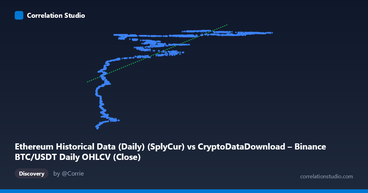
Ethereum Historical Data (Daily) (SplyCur) vs CryptoDataDownload – Binance BTC/USDT Daily OHLCV (Close)

Pearson correlation (r): 0.6738
Spearman correlation: 0.8228
p-value: 0
Sample size (n): 3191
95% confidence interval: 0.6544 to 0.6924
Granger causality: None
Granger optimal lag: 10
Time coverage: 2017-08-17 to 2026-05-20

AI analysis

Analysis of the Relationship Between X (Ethereum Circulating Supply) and Y (BTC/USDT Close Price)

Note on variable labeling: The axis metadata appears mismatched/swapped — X is described as "Ethereum SplyCur" while Y is described as "BTC/USDT Close." Given the sample data (X ranges ~3,189–124,658; Y ranges ~$94M–$121M), it's more likely that X represents a Bitcoin-related supply/count metric and Y represents a price series scaled oddly, or there's a data-processing artifact (e.g., Y values look like they could be off by a factor, since BTC has never traded at $94–121 million). Treat the following analysis as describing the statistical relationship between the two series as given, independent of label interpretation.

1. What the Visualization Reveals

The scatterplot shows a clear non-linear, saturating relationship rather than a simple straight line. At low X values (roughly 3,000–20,000), Y rises steeply from ~94M to ~113M. Beyond X ≈ 30,000–40,000, Y plateaus and hovers tightly in a narrow band (~118M–122M) regardless of further increases in X out to 124,000+. This produces a classic logarithmic or square-root-shaped curve: rapid initial growth followed by diminishing returns/flattening.

2. Strength, Direction, and Statistical Confidence

The Pearson correlation (r = 0.674) indicates a moderate-to-strong positive linear association, but r² = 0.454 means the linear model only explains about 45% of the variance in Y — the remaining 55% is unexplained by a straight-line fit. The 95% CI [0.654, 0.692] is tight given the large sample (n=3,191), and the p-value of ~0 confirms the correlation is highly statistically significant — this relationship is not due to chance. However, statistical significance here reflects sample size more than model quality; the r² ceiling suggests linearity is not the right functional form. The note that Spearman ρ exceeds Pearson r reinforces this: the rank-order relationship is stronger than the linear one, confirming a monotonic but curved (likely logarithmic) relationship would fit better and explain more variance.

Critically, the Granger causality tests show no significant predictive direction in either direction (X→Y: p=0.916; Y→X: p=0.383). This means neither series' past values help forecast the other's future values at any of the tested lags. Combined with a strong contemporaneous correlation, this pattern is typical of two variables that are both driven by a common underlying trend (e.g., time, or market-wide crypto growth) rather than one causing the other. This is an important caveat: correlation without Granger causality often signals confounding by a shared time trend, not a causal or leading/lagging relationship.

3. Notable Patterns and Outliers

- Two-regime structure: A steep-rise regime (X < ~25,000) and a flat/plateau regime (X ~30,000). This is the dominant non-linear feature. - Vertical clustering at low X: Points like (4,378 → 94.9M), (6,390 → 100.4M), (10,237 → 97.3M) show substantial Y variance even at similar low X values, suggesting noise or an additional factor at play in the early regime. - Plateau band: From X≈30,000 to X≈124,000, Y compresses into a tight 118M–122M range, indicating the relationship saturates — Y is nearly insensitive to X in this range. - No obvious extreme outliers, but the low-X cluster has higher relative scatter (heteroscedasticity) compared to the tighter high-X plateau.

4. Confounding Factors and Caveats

- Shared time trend: Both series likely trend upward over the 2017–2026 window due to broad crypto market growth, adoption, and macro cycles. This is the most probable driver of the correlation, not a direct causal link — consistent with the null Granger result. - Label/unit inconsistency: The described Y variable (BTC close price) is inconsistent with the observed value range (~$94–121 million), suggesting a data pipeline issue (wrong column mapping, incorrect scaling, or aggregation). This must be resolved before drawing domain conclusions. - Non-stationarity: Both crypto price/supply series are typically non-stationary (trending), which can inflate Pearson r and produce misleading "significant" p-values — this is a well-known issue in time-series correlation analysis and matches the Granger non-causality finding. - Autocorrelation: Daily financial/network data is highly autocorrelated, violating the independence assumption behind the reported p-values; effective sample size is smaller than n=3,191 suggests.

5. Actionable Insights

1. Fit a non-linear model (logarithmic, square-root, or piecewise/segmented regression) — given Spearman Pearson and the visible plateau, this should meaningfully improve variance explained beyond 45%. 2. Verify data labeling/scaling — confirm whether Y truly represents BTC close price or another metric, as the current values don't match known BTC price history. 3. Test for cointegration (e.g., Engle-Granger or Johansen test) rather than relying on levels correlation, since both series appear non-stationary and trend-driven. 4. Difference or detrend both series before re-testing correlation and Granger causality — this isolates short-term co-movement from shared long-term trend and gives a cleaner causal read. 5. Segment the analysis by regime (low-X vs. plateau region) to understand what drives the steep early relationship versus the flat later one — they may reflect fundamentally different market phases or supply dynamics.

X dataset: CryptoDataDownload – Binance BTC/USDT Daily OHLCV

Y dataset: Ethereum Historical Data (Daily)

Part of experiment: Bitcoin - CryptoDataDownload – Binance BTC/USDT Daily OHLCV vs Ethereum Historical Data (Daily)