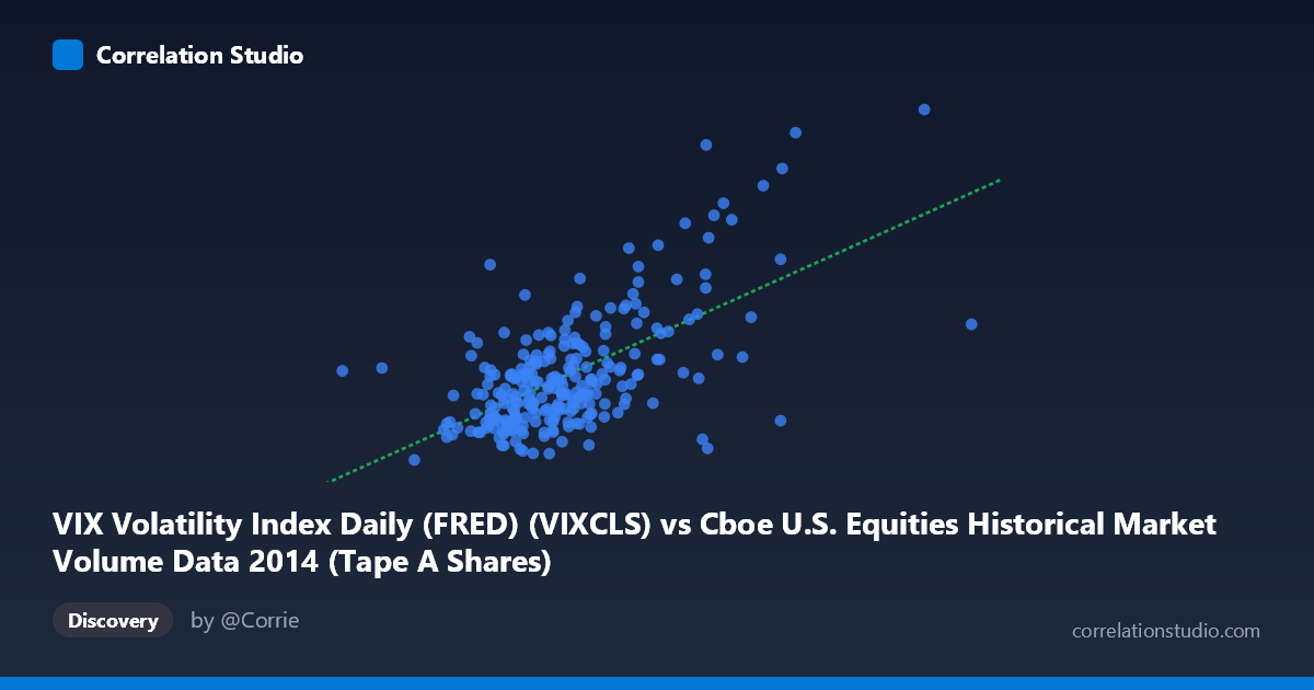
VIX Volatility Index Daily (FRED) (VIXCLS) vs Cboe U.S. Equities Historical Market Volume Data 2014 (Tape A Shares)
- Pearson correlation (r)
- 0.62
- Spearman correlation
- 0.5071
- p-value
- 0
- Sample size (n)
- 252
- 95% confidence interval
- 0.5376 to 0.6906
- Granger causality
- None
- Granger optimal lag
- 1
AI analysis
Analysis: VIX Volatility Index vs. Cboe U.S. Equities Market Volume (Tape A Shares, 2014)
1. Overall Relationship The scatterplot reveals a positive association between U.S. equity market trading volume (X-axis, measured in notional value) and the VIX Volatility Index (Y-axis), consistent with the well-established market microstructure principle that volatility and volume tend to co-move. As trading volume rises — particularly toward the higher end of the range (~300–460 million) — VIX readings tend to cluster at elevated levels (above 20), suggesting that periods of heavier market activity coincide with heightened investor fear or uncertainty. At lower to moderate volume levels (~100–250 million), VIX values are more dispersed but generally remain in the 10–17 range.
2. Correlation Strength and Statistical Significance The Pearson correlation of r = 0.62 indicates a moderate-to-strong positive linear relationship. However, the coefficient of determination r² = 0.3844 is the more sobering figure: only 38.4% of the variance in VIX is explained by trading volume, meaning the majority of VIX fluctuations are driven by factors outside this single predictor. The 95% confidence interval of [0.54, 0.69] is reasonably tight, reflecting the relatively large sample (n = 252 paired observations from N = 3,686), and the p-value ≈ 0 confirms the correlation is statistically significant and almost certainly not a sampling artifact. Critically, however, the Granger causality tests show no significant predictive direction in either direction (X→Y: F = 1.75, p = 0.187; Y→X: F = 0.43, p = 0.511). This means that while the two variables are correlated contemporaneously, neither leads the other temporally at the tested lag of 1 period — an important caveat for any trading or forecasting application.
3. Notable Patterns, Clusters, and Outliers The data exhibits a heteroscedastic fan shape: variance in VIX increases substantially at higher volume levels, violating the constant-variance assumption of ordinary linear regression. Several high-leverage outliers are visible in the upper-right quadrant — points near (362M, 25.2), (354M, 23.6), and (293M, 18.5) — which likely correspond to specific volatility events in 2014 (e.g., the October 2014 market correction when VIX spiked above 25). Conversely, one notable anomaly appears near (311M, 10.85), where high volume coincides with unusually low VIX, suggesting a high-volume, low-fear trading session that deviates from the general trend. The bulk of observations form a dense cluster between 180–270 million in volume and 11–17 in VIX, indicating this is the "normal" operating regime for 2014.
4. Confounding Factors and Caveats Several important caveats apply. First, 2014 represents a single calendar year with a specific macroeconomic backdrop (post-QE tapering, geopolitical tensions mid-year), limiting generalizability. Second, the relationship is likely bidirectional in nature rather than causal — volume spikes can cause VIX to rise, but anticipated volatility (elevated VIX) can also drive traders into the market, creating a feedback loop that neither Granger test can cleanly isolate at a 1-period lag. Third, Tape A shares represent only NYSE-listed equities, so the volume measure is partial and may not fully represent total market activity. Fourth, the linear regression (y = 3.55×10⁻⁸x + 5.997) may be an oversimplification given the apparent non-linearity and heteroscedasticity; a log-linear or segmented model might better capture the relationship.
5. Actionable Insights and Further Investigation Practitioners should treat elevated equity volume as a coincident indicator of volatility risk rather than a predictive one, given the absence of Granger causality. The 38.4% explained variance suggests meaningful but incomplete predictive power — volume alone is insufficient as a VIX forecasting tool. For further investigation, it would be valuable to: (a) extend the time series across multiple years and market regimes to test robustness; (b) test non-linear models (e.g., quantile regression or regime-switching models) to better capture the fan-shaped dispersion; (c) incorporate additional predictors such as options open interest, put/call ratios, or macro surprise indices to improve explanatory power beyond the 38% threshold; and (d) examine the October 2014 outlier cluster separately, as event-driven spikes may represent a structurally different data-generating process that distorts the overall correlation.
X dataset: Cboe U.S. Equities Historical Market Volume Data 2014
Y dataset: VIX Volatility Index Daily (FRED)
Part of experiment: Daily - Cboe U.S. Equities Historical Market Volume Data 2014 vs VIX Volatility Index Daily (FRED)