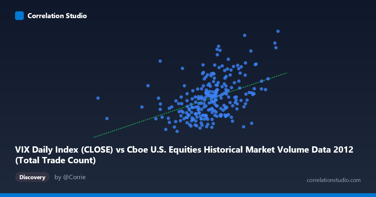
VIX Daily Index (CLOSE) vs Cboe U.S. Equities Historical Market Volume Data 2012 (Total Trade Count)

Pearson correlation (r): 0.4374
Spearman correlation: 0.459
p-value: 0
Sample size (n): 250
95% confidence interval: 0.3314 to 0.5326
Granger causality: None
Granger optimal lag: 1

AI analysis

Analysis: VIX Daily Index vs. Total Trade Count (2012)

Relationship Overview

The scatterplot reveals a moderate positive relationship between the Cboe VIX Daily Index (close prices) and the Total Trade Count in U.S. equities markets during 2012. As VIX values increase — reflecting heightened market volatility and investor fear — the total number of trades tends to rise as well. This is broadly consistent with market microstructure theory: periods of elevated uncertainty drive increased trading activity as investors rebalance portfolios, hedge positions, or react to news. The linear regression equation (y = 4.68E-06x + 10.09) suggests that for every unit increase in VIX, trade count increases marginally, though the relationship is far from deterministic.

Correlation Strength and Statistical Significance

The Pearson correlation of r = 0.4374 indicates a moderate positive association, but the explanatory power is notably limited: r² = 0.1914, meaning VIX explains only about 19.1% of the variance in total trade count, leaving roughly 81% attributable to other factors. The 95% confidence interval of [0.3314, 0.5326] confirms the correlation is meaningfully positive and reasonably well-bounded, not straddling zero. The p-value of 4.15E-13 — extraordinarily small across a paired sample of n = 250 drawn from a population of N = 3,750 — makes it statistically robust; this is almost certainly not a chance finding. However, statistical significance should not be conflated with practical significance: the moderate r and low r² suggest VIX alone is a weak predictor of trade volume in isolation. Critically, the Granger causality tests return no significant directional predictability in either direction (X→Y: F = 0.166, p = 0.684; Y→X: F = 0.218, p = 0.641). This means that, at the tested lag of 1 period, neither variable reliably forecasts the other temporally — the contemporaneous correlation does not translate into a usable lead-lag trading signal.

Patterns, Clusters, and Outliers

The sample points reveal several noteworthy structural features. The bulk of observations cluster in the VIX range of roughly 1.4M–1.9M (X-axis) with trade counts concentrated between 15 and 20 (Y-axis), forming a dense central cloud with moderate upward drift. However, there are visible outlier observations at higher trade counts (e.g., points near 22–26 on the Y-axis), which appear dispersed across a range of VIX values rather than neatly following the regression line — suggesting these high-activity days may be driven by idiosyncratic events rather than VIX alone. Notably, several high-Y outliers appear at moderate X values (e.g., ~1,577K VIX with trade count ~22.22; ~1,712K with ~23.56), while some high-X observations (e.g., ~2,036K) correspond to relatively low trade counts (~14.5), directly contradicting the general trend. This scatter and the presence of points far from the regression line reinforce the modest r².

Confounding Factors and Caveats

Several important caveats apply. First, the axis labels appear swapped relative to convention: the dataset description places VIX on the X-axis but sourced from the "Market Volume" dataset, and Trade Count on the Y-axis sourced from the "VIX" dataset — this labeling inconsistency warrants verification before drawing firm conclusions. Second, 2012 was a relatively low-volatility year (post-2008 normalization), which compresses the VIX range and may understate the true relationship observable across a fuller volatility cycle. Third, algorithmic and high-frequency trading activity can inflate trade counts independently of VIX, introducing noise. Fourth, seasonality, earnings seasons, and macro events (e.g., European debt crisis developments, U.S. election) likely drove simultaneous spikes in both variables, creating spurious correlation episodes. Finally, the absence of Granger causality at lag 1 may reflect the need to test longer lag structures or intraday data to detect any genuine predictive relationship.

Actionable Insights and Further Investigation

Despite the moderate correlation, several practical steps could deepen this analysis. Multivariate modeling incorporating additional predictors — such as bid-ask spreads, options open interest, or macro news indicators — would likely substantially improve the explained variance beyond the current 19.1%. Researchers should test Granger causality at longer lags (2–5 periods) and consider rolling-window correlations to assess whether the VIX–volume relationship strengthens during specific market regimes (e.g., high-stress vs. calm periods). A quantile regression approach could help determine whether the relationship is stronger at the extremes of VIX (tail events) than in the middle, which the scatterplot hints at. Finally, given the data covers only 2012, extending the analysis across multiple years — including 2008–2009 and 2020 — would provide a more robust and generalizable picture of how volatility and trading activity co-move across full market cycles.

X dataset: Cboe U.S. Equities Historical Market Volume Data 2012

Y dataset: VIX Daily Index

Part of experiment: Daily - Cboe U.S. Equities Historical Market Volume Data 2012 vs VIX Daily Index