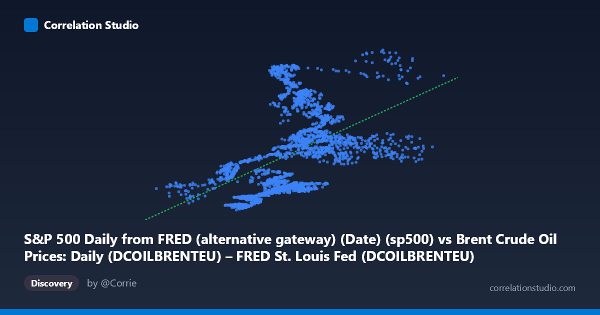
S&P 500 Daily from FRED (alternative gateway) (Date) (sp500) vs Brent Crude Oil Prices: Daily (DCOILBRENTEU) – FRED St. Louis Fed (DCOILBRENTEU)
- Pearson correlation (r)
- 0.4795
- Spearman correlation
- 0.5862
- p-value
- 0
- Sample size (n)
- 2475
- 95% confidence interval
- 0.4485 to 0.5093
- Granger causality
- None
- Granger optimal lag
- 9
AI analysis
Analysis: S&P 500 vs. Brent Crude Oil Prices (2016–2026)
1. Overall Relationship Revealed
The scatterplot reveals a moderate positive association between daily Brent crude oil prices (X-axis) and S&P 500 index values (Y-axis) across roughly a decade of paired daily observations. As crude oil prices rise from ~$9 to ~$138 per barrel, S&P 500 values tend to climb from roughly 2,000 to 7,500 points. However, the scatter is wide and visually striking — at any given oil price level, S&P 500 values span an enormous range (often 2,000–3,000 index points), making clear that oil price alone is a far from deterministic predictor of equity market levels. The linear regression line (y = 34.87x + 1,515.34) captures a general upward trend, but the cloud of points around it betrays substantial unexplained variation.
2. Correlation Strength, Direction, and Causality
The Pearson r of 0.4795 indicates a moderate positive correlation, statistically significant (p ≈ 0, N = 2,475), with a tight 95% confidence interval of [0.449, 0.509] confirming the estimate is stable and not a sampling artifact. However, r² = 0.2299 tells the more important story: oil prices explain only about 23% of the variance in S&P 500 levels, leaving 77% attributed to other forces entirely. This is a critical practical caveat — while the relationship is real, it is weak as a predictive tool. The fact that Spearman ρ exceeds Pearson r is a notable flag, suggesting the true relationship is better described by a monotonic but non-linear function (e.g., logarithmic or polynomial) rather than a straight line, meaning the linear model systematically under- or over-estimates at the extremes.
The Granger causality results are unambiguous in their null finding: neither X→Y (F = 1.56, p = 0.12) nor Y→X (F = 0.97, p = 0.46) reaches significance at the optimal lag of 9 periods. This means that past oil prices do not significantly help predict future S&P 500 values, and vice versa, in this dataset. The observed correlation is therefore a contemporaneous, likely co-movement relationship rather than a directional predictive one — both variables may be responding to shared underlying drivers rather than causally influencing each other.
3. Notable Patterns, Clusters, and Outliers
Several structural features stand out in the sample points and implied distribution. There appears to be a dense cluster in the mid-range (oil: $45–$85; S&P: 2,500–5,000), representing the bulk of post-2016 trading days under relatively normal macroeconomic conditions. High-leverage outliers are visible at the extremes: points like (119.03, 6,824.66) and (74.52, 5,618.26) sit well above the regression line, while (55.89, 2,296.68) and (46.69, 2,037.41) sit below it, suggesting regime-dependent behavior. The very low oil prices (below $30) almost certainly reflect the COVID-19 crash of early 2020, when both oil and equities collapsed simultaneously — a structural break that may artificially inflate the correlation by adding extreme co-downturns. Conversely, high-equity/moderate-oil combinations (post-2023 AI-driven rally with stabilized oil) pull the relationship away from linearity, contributing to the Spearman Pearson divergence.
4. Confounding Factors and Interpretive Caveats
Several important confounds compromise any causal interpretation. Secular time trends are the most significant: both S&P 500 and oil prices trended upward over much of this period due to inflation, dollar dynamics, and economic growth — their correlation may largely reflect shared temporal drift rather than a structural link. Macroeconomic regimes (pre-COVID expansion, COVID crash, post-COVID recovery, rate-hiking cycle) create distinct data clusters that behave differently within each period, violating the stationarity assumptions underlying simple correlation. Currency effects matter too, as Brent is priced in USD; a weakening dollar simultaneously boosts both oil prices and multinational S&P 500 earnings. Additionally, the axes appear swapped in the dataset labels (the description notes oil on X but the dataset names reference each other's series), warranting verification of column assignment before drawing firm conclusions.
5. Actionable Insights and Further Investigation
Given the moderate but non-causal relationship, practitioners should avoid using oil prices as a standalone equity signal. Recommended next steps include: (1) fitting a logarithmic or polynomial regression model to better capture the non-linear monotonic relationship flagged by the Spearman divergence; (2) segmenting by macroeconomic regime (using recession indicators, Fed policy phases, or volatility regimes via VIX) to test whether the correlation strengthens or reverses within coherent subperiods; (3) running a partial correlation analysis controlling for USD index and global growth proxies (e.g., PMI data) to isolate whether oil-equity co-movement survives after removing common macro drivers; (4) extending Granger causality testing with longer lags or a VAR framework incorporating intermediate variables like inflation expectations; and (5) examining sector-level S&P 500 data (energy vs. technology vs. consumer) since energy stocks would be expected to show a much stronger oil correlation, while tech-heavy indices might show an inverse relationship — aggregation may be masking these opposing signals.
X dataset: Brent Crude Oil Prices: Daily (DCOILBRENTEU) – FRED St. Louis Fed
Y dataset: S&P 500 Daily from FRED (alternative gateway) (Date)
Part of experiment: Daily - Brent Crude Oil Prices: Daily (DCOILBRENTEU) – FRED St. Louis Fed vs S&P 500 Daily from FRED (alternative gateway) (Date)