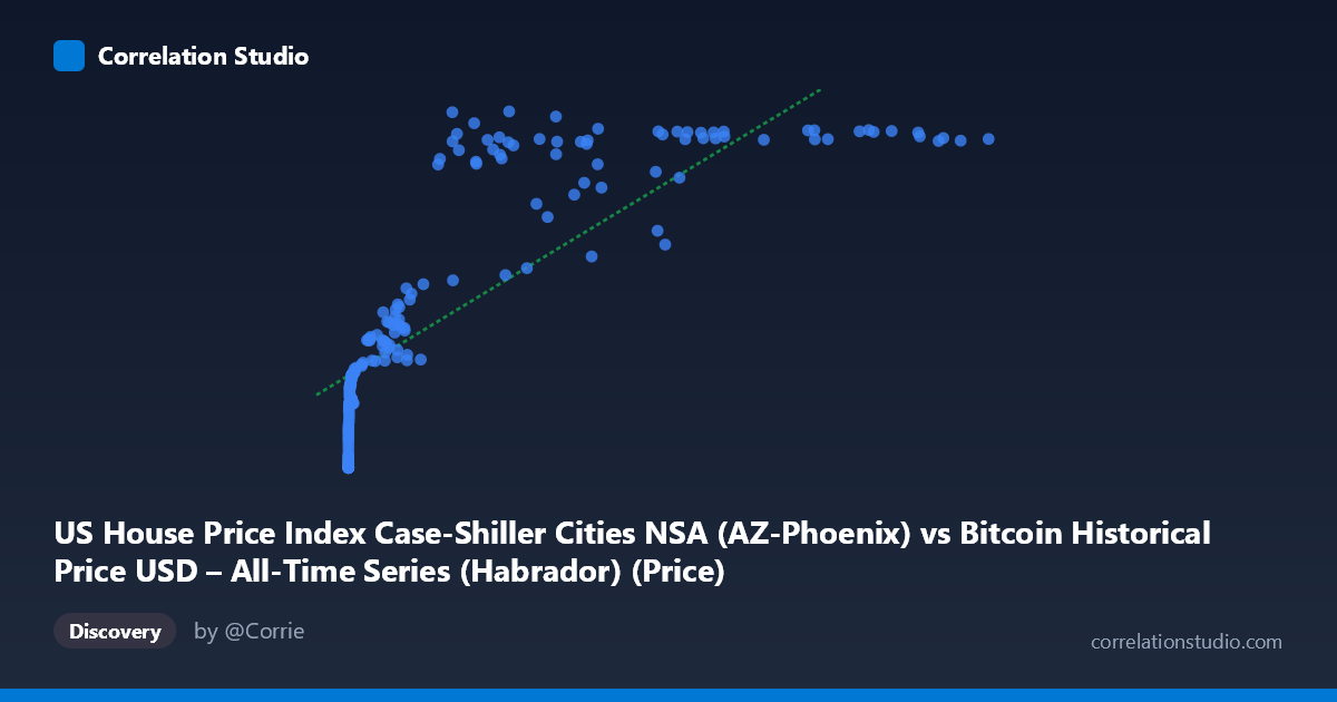
US House Price Index Case-Shiller Cities NSA (AZ-Phoenix) vs Bitcoin Historical Price USD – All-Time Series (Habrador) (Price)
- Pearson correlation (r)
- 0.8123
- Spearman correlation
- 0.9582
- p-value
- 0
- Sample size (n)
- 187
- 95% confidence interval
- 0.757 to 0.856
- Granger causality
- None
- Granger optimal lag
- 9
AI analysis
Analysis: Bitcoin Price vs. Case-Shiller Phoenix Home Price Index
1. Relationship Overview
The scatterplot depicts a strongly positive but distinctly non-linear relationship between Bitcoin's historical USD price and the Phoenix Case-Shiller Home Price Index. Rather than a straight-line trend, the data shows a compressed, logarithmic-style pattern: Y (the home price index) rises quickly at low X values, then flattens into a plateau around 320-330 as X grows into the tens of thousands and beyond. This is visible in the sample points — indices near 100-170 occur when Bitcoin is under ~$1,000, but the index saturates near 320-330 for Bitcoin prices ranging anywhere from $27,000 to $118,000, indicating a ceiling effect rather than continued proportional growth.
2. Strength, Direction, and Statistical Confidence
The Pearson correlation (r = 0.812, r² = 0.660) indicates a strong positive association, with 66% of the variance in Y statistically explained by X in a linear framework. However, given 187 paired observations, the 95% CI [0.757, 0.860] is reasonably tight, and the p-value of ~0 confirms the correlation is highly unlikely to be due to chance. That said, correlation strength should not imply causation or predictive power: the Granger causality tests show no significant directional relationship in either direction (X→Y: p=0.70; Y→X: p=0.84) at the tested lag structure. This means neither variable's historical values reliably help forecast the other's future values in a time-series sense — the association is likely driven by both series independently trending upward over the same historical period (2010-2026), a classic case of spurious correlation from shared time trends rather than genuine interdependence.
3. Notable Patterns and Outliers
Several features stand out: - Saturation/plateau: Once Bitcoin exceeds ~$25,000-30,000, the home price index consistently clusters in the 320-330 range regardless of further Bitcoin price increases (e.g., $34,855 → 280.47; $118,670 → 324.73), suggesting the true relationship is asymptotic/logarithmic, not linear. - Low-X density: A large cluster of points exists at very low Bitcoin prices (X < 20), reflecting Bitcoin's early years (2010-2013), where Y ranges narrowly between 100-130. - Mid-range volatility: Notable non-monotonic dips exist — e.g., X=45,092 gives Y=244.55, and X=58,724 gives Y=252.66, both lower than neighboring points with smaller X values (X=44,354→323.78), indicating temporary divergences, likely reflecting real estate cycles (2008 crash recovery, 2020 COVID dip) that don't track Bitcoin's price swings at all. - The Spearman ρ Pearson r explicitly confirms the rank-order relationship is stronger than the linear fit, reinforcing that a log or polynomial model fits better.
4. Confounding Factors and Caveats
This correlation is very likely spurious or confounded by time itself. Both Bitcoin price and US home prices have exhibited long-term secular uptrends over the 2010-2026 window due to entirely separate macro forces: Bitcoin's growth reflects adoption, speculation, and crypto-market cycles, while Case-Shiller indices reflect mortgage rates, housing supply constraints, wage growth, and regional Phoenix market dynamics (notably the post-2020 pandemic-driven housing boom). Any two monotonically trending time series will show high correlation without genuine causal linkage. Additionally, Bitcoin's extreme right-skewed distribution (X range 0.06 to 118,670, stdev 29,663 vs. mean 20,037) means the linear regression is heavily influenced by a few high-value points, while the bulk of observations sit near zero — violating linear regression assumptions and inflating apparent fit.
5. Suggested Next Steps
1. Detrend both series (e.g., using differencing, year-over-year % change, or removing time trend via regression residuals) and re-test correlation — this is the standard way to distinguish genuine co-movement from shared trend artifacts. 2. Re-fit using log(X) given the clear logarithmic saturation pattern — this should substantially improve model fit and better reflect the true functional relationship. 3. Treat Granger non-significance as decisive: given no lead-lag predictive relationship exists, avoid using Bitcoin price as a leading indicator for regional home prices (or vice versa) in forecasting models. 4. Consider controlling for common macro drivers (Fed interest rates, inflation, USD strength) that could simultaneously influence both housing and crypto markets, to test whether the correlation persists as a third-variable effect once these are held constant.
X dataset: Bitcoin Historical Price USD – All-Time Series (Habrador)
Y dataset: US House Price Index Case-Shiller Cities NSA
Part of experiment: Bitcoin - Bitcoin Historical Price USD – All-Time Series (Habrador) vs US House Price Index Case-Shiller Cities NSA