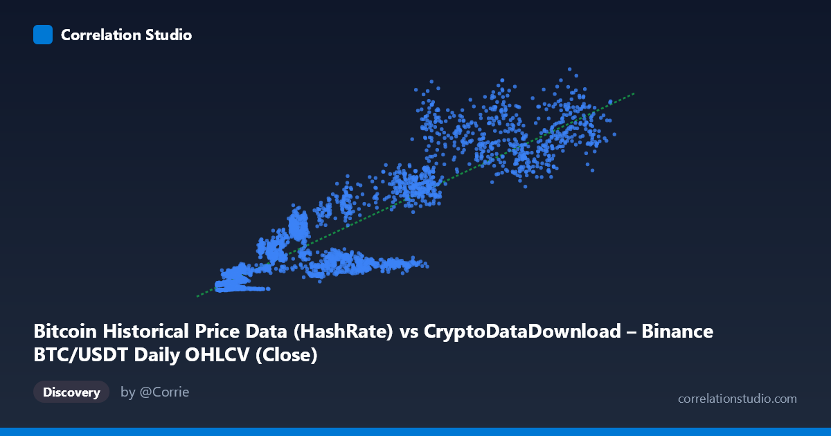
Bitcoin Historical Price Data (HashRate) vs CryptoDataDownload – Binance BTC/USDT Daily OHLCV (Close)

Pearson correlation (r): 0.8909
Spearman correlation: 0.8817
p-value: 0
Sample size (n): 3191
95% confidence interval: 0.8835 to 0.8978
Granger causality: None
Granger optimal lag: 10

AI analysis

Analysis: Bitcoin Hash Rate vs. Price Relationship

1. What the Visualization Reveals

The scatterplot shows a strong positive association between Bitcoin's network hash rate (X-axis) and its closing price (Y-axis). As hash rate increases from roughly 3,000 to 125,000 units, price generally rises from single-digit millions to over a billion (in whatever base units the Y-axis represents). The relationship is not a tight linear line but rather a widening cone/fan shape — variance in price grows substantially as hash rate increases, indicating heteroscedasticity rather than a uniform linear relationship across the full range.

2. Strength, Direction, and Statistical Confidence

The correlation coefficient (r = 0.891) indicates a strong positive linear relationship, with r² = 0.794 meaning hash rate statistically "explains" about 79% of the variance in price — leaving roughly 21% unexplained by this linear model alone. The narrow 95% CI [0.884, 0.898] and p-value of 0 (effectively p < 0.0001) confirm this correlation is highly statistically significant and precisely estimated, not a artifact of sampling noise, given the large sample (n=3,191).

However, statistical correlation is not causation, and the Granger causality tests make this explicit: neither variable Granger-causes the other at conventional significance levels (X→Y: p=0.49; Y→X: p=0.165). This means past values of hash rate do not significantly improve prediction of future price beyond price's own history, and vice versa. Practically, this suggests both variables are likely responding to a common underlying driver (e.g., market cycles, adoption trends) rather than one mechanically leading the other in a exploitable temporal sequence — at least at the lag structure tested (10 periods).

3. Notable Patterns and Non-Linear Features

Several features stand out: - Fan-shaped dispersion: At low hash rates (<15,000), price values cluster tightly near the low end. At high hash rates (60,000), price values scatter widely — from ~500M to over 1.3B — suggesting hash rate alone is a weaker predictor of price during high-network-security periods, likely because price is also driven by demand-side speculation, macro conditions, and halving cycles independent of hash rate. - Sub-clusters: There appear to be distinct bands (e.g., prices around 100–150M co-occurring with hash rates in the 50,000–60,000 range alongside other points near hash rate 60,000 with price 500M), hinting at regime shifts or different market cycles/eras occupying similar hash rate levels but very different price levels — consistent with Bitcoin's boom-bust cycles (2018 bear market vs. 2021 bull run vs. 2024-2025 dynamics). - Non-linearity: The relationship looks like it could be better fit by a power/log curve rather than pure linear, since price growth appears to accelerate faster than hash rate in certain regions (typical of exponential-style crypto price action).

4. Confounding Factors and Caveats

Both hash rate and price are jointly driven by external factors: overall crypto market sentiment, Bitcoin halving events (which reduce mining rewards and indirectly affect both hash rate economics and price), macroeconomic conditions (interest rates, dollar strength), regulatory news, and mining hardware efficiency improvements. Critically, hash rate itself is partly a function of price (miners deploy more hardware when mining is profitable, i.e., when price is high) — creating potential reverse endogeneity that a simple correlation cannot disentangle. Additionally, this is time-series data (2017–2026), so both variables are non-stationary and trending upward together over time; such "spurious correlation via common trend" is common in crypto datasets and elevates r² without necessarily indicating a direct mechanistic link. The Granger causality results support this concern — the correlation may simply reflect codependence on time/trend rather than either variable driving the other.

5. Recommendations for Further Investigation

- De-trend or difference the series (e.g., use returns/percentage changes rather than levels) before re-running correlation and Granger tests, since non-stationary trending data inflates naive correlation. - Test non-linear models (log-log or power-law regression) given the fan-shaped/exponential-looking dispersion — this may explain more variance than the linear r²=0.794. - Segment by market era (bear vs. bull cycles, pre/post-halving) to see if the hash-rate/price relationship is stable or regime-dependent. - Explore additional lag structures in Granger causality (beyond the 10-period optimum) and test with weekly/monthly aggregation to rule out lag-mismatch issues. - Incorporate a third variable (e.g., mining difficulty, transaction volume, or macro indices) to test whether hash rate and price are both proxies for overall network/market growth rather than causally linked.

X dataset: CryptoDataDownload – Binance BTC/USDT Daily OHLCV

Y dataset: Bitcoin Historical Price Data

Part of experiment: Bitcoin - CryptoDataDownload – Binance BTC/USDT Daily OHLCV vs Bitcoin Historical Price Data