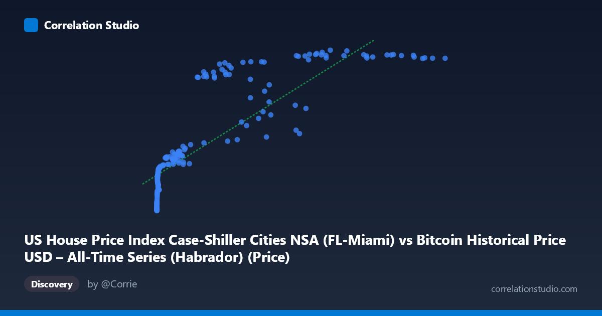
US House Price Index Case-Shiller Cities NSA (FL-Miami) vs Bitcoin Historical Price USD – All-Time Series (Habrador) (Price)
- Pearson correlation (r)
- 0.8442
- Spearman correlation
- 0.9682
- p-value
- 0
- Sample size (n)
- 191
- 95% confidence interval
- 0.7978 to 0.8806
- Granger causality
- None
- Granger optimal lag
- 9
- Time coverage
- 2010-08-01 to 2026-06-01
- Recomputed on refreshed data
- 2026-10-24 (r was 0.8391)
AI analysis
Analysis: Bitcoin Price vs. Miami Case-Shiller Home Price Index
1. What the Visualization Reveals
The scatterplot shows a strong positive association between Bitcoin's historical USD price and the Miami Case-Shiller Home Price Index. However, the relationship is clearly non-linear — data points trace a curve that resembles a logarithmic or saturating function rather than a straight line. At low Bitcoin values (under ~$1,000), the Miami index climbs steeply from ~137 to ~230, then the curve flattens considerably as Bitcoin prices rise into the tens of thousands, with the index compressing into a narrower band (roughly 280–444) despite Bitcoin spanning from $10,000 to $118,000+.
2. Strength, Direction, and Uncertainty
The Pearson correlation (r = 0.8345) indicates a strong positive linear relationship, with r² = 0.6964 meaning the linear model explains about 70% of the variance in the Miami index — a substantial but incomplete fit given the noted non-linearity (Spearman ρ exceeding Pearson r confirms curvature). The 95% CI [0.785, 0.873] is fairly tight and excludes zero, and the p-value of 0 confirms this correlation is statistically robust and not due to chance, given n=187. Critically, however, the Granger causality test shows no predictive direction in either direction (Bitcoin→HPI: p=0.76; HPI→Bitcoin: p=0.76). This means that despite the strong contemporaneous correlation, neither variable's past values help forecast the other's future values — the relationship is likely driven by a shared external trend (e.g., both series growing over the same historical period) rather than one causing or leading the other.
3. Notable Patterns and Outliers
Several structural features stand out: - Two regimes: A steep early-growth phase (X < $1,000) where small Bitcoin increases correspond to large jumps in the index, and a flatter, saturated phase (X $20,000) where the index hovers in a narrower high range. - Vertical scatter at high X: At similar Bitcoin prices (e.g., ~$57,000–$62,000), the index varies substantially (288 to 441), suggesting time-order effects — likely early 2021 vs. later 2021/2022 observations — rather than a stable functional relationship. - Compression near the ceiling: Many high-Bitcoin-price points cluster near index values of 435–444, suggesting the housing index may be approaching a plateau or reflecting market saturation/seasonality independent of BTC price.
4. Confounding Factors and Caveats
This is almost certainly a spurious or trend-driven correlation rather than a causal economic relationship. Both Bitcoin and the Miami housing index have exhibited strong secular upward trends over the 2010–2026 window, driven by unrelated macro forces: near-zero interest rates (2010s), pandemic-era stimulus, Miami-specific migration/demand booms, and independent Bitcoin adoption/speculation cycles. Any two upward-trending time series will show high correlation without genuine linkage. The lack of Granger causality strongly supports this interpretation — there's no evidence of information flow between the series. Additionally, non-stationarity (both series trending) violates assumptions of standard correlation/regression and can inflate r artificially.
5. Suggestions for Further Investigation
- Detrend both series (e.g., using year-over-year returns or first differences) and recompute correlation to test whether the relationship holds in growth-rate terms — this often eliminates spurious trend-correlation. - Fit a log-log or log-linear model given the evident logarithmic curvature (log(X) vs Y) to improve fit quality and better characterize the saturating relationship. - Introduce a common macro factor (e.g., M2 money supply, federal funds rate, or general inflation) as a control variable to test if it better explains both series' movements. - Given no Granger causality, avoid using one series to forecast the other; instead, treat this as two assets responding similarly to a shared macroeconomic environment rather than a tradable causal signal.
X dataset: Bitcoin Historical Price USD – All-Time Series (Habrador)
Y dataset: US House Price Index Case-Shiller Cities NSA
Part of experiment: Bitcoin - Bitcoin Historical Price USD – All-Time Series (Habrador) vs US House Price Index Case-Shiller Cities NSA