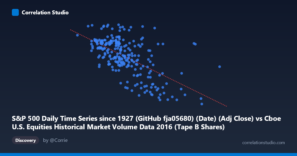
S&P 500 Daily Time Series since 1927 (GitHub fja05680) (Date) (Adj Close) vs Cboe U.S. Equities Historical Market Volume Data 2016 (Tape B Shares)

Pearson correlation (r): -0.6107
Spearman correlation: -0.5802
p-value: 0
Sample size (n): 252
95% confidence interval: -0.6827 to -0.5269
Granger causality: None
Granger optimal lag: 1

AI analysis

Analysis: S&P 500 Price vs. Cboe Tape B Share Volume (2016)

Relationship Overview The scatterplot reveals a moderate negative relationship between the S&P 500 adjusted closing price (X-axis) and Cboe Tape B share volume (Y-axis) across 252 trading days in 2016. As the S&P 500 index level rises, Tape B share volume tends to decline, and vice versa. This inverse pattern is visually apparent as a downward-sloping cloud of points, consistent with the fitted regression line: y = −2.046×10⁻⁶x + 2313.93. In practical terms, higher equity index levels in 2016 were associated with quieter, lower-volume trading sessions on Tape B exchanges, while lower index levels — particularly in the year's early months — coincided with elevated trading activity.

Correlation Strength and Statistical Significance The Pearson correlation of r = −0.6107 reflects a moderate-to-strong negative association, and the r² of 0.3729 indicates that roughly 37.3% of the variance in Tape B share volume is statistically explained by the S&P 500 price level. While meaningful, this also means that nearly 63% of volume variance remains unexplained by price alone, pointing to other influential factors. The 95% confidence interval of [−0.6827, −0.5269] is relatively tight and does not contain zero, and the p-value is effectively zero (p ≈ 0), confirming this relationship is highly unlikely to be a product of random chance given the sample of 252 paired observations drawn from a population of N = 3,622. However, the Granger causality tests complicate any causal narrative: neither direction (X→Y nor Y→X) achieves significance at a one-period lag (F = 0.52, p = 0.47 and F = 0.65, p = 0.42, respectively). This means that, statistically, neither variable reliably predicts the next day's movement in the other — the correlation reflects a contemporaneous structural relationship rather than a temporal lead-lag dynamic.

Notable Patterns, Clusters, and Outliers Several structural features are worth noting. The data exhibits a broad horizontal dispersion at mid-range X values (~85M–115M), suggesting considerable volume variability even when the S&P 500 is within its typical 2016 range. At the lower end of the X-axis (index levels below ~75M, corresponding to early 2016 market stress), volume spikes are visible, consistent with panic-driven or volatility-induced trading surges. A small cluster of high-volume outliers appears around Tape B values of ~2,260–2,271, including notably the point near (78.9M, 2265) and (130.8M, 2262), which deviate from the main trend — the latter being particularly unusual as it combines a relatively high index level with very high volume. At the upper-right of the X-axis, points corresponding to the post-election S&P 500 rally (late 2016, ~170M+) show markedly suppressed Tape B volume, reinforcing the inverse pattern. The vertical spread at any given X value is substantial (~200+ share units), suggesting the relationship is real but noisy.

Confounding Factors and Interpretive Caveats This correlation likely reflects a well-documented market microstructure phenomenon: elevated volatility and fear (low prices) drive higher trading volumes, while calm, rising markets generate complacency and lower turnover — sometimes called the volume-volatility relationship or a manifestation of the VIX-volume linkage. Importantly, the X-axis variable here is an index price level, not a return or volatility measure, so the causal mechanism is indirect at best. Tape B specifically covers NYSE MKT, NYSE Arca, and regional exchanges, so its volume dynamics may differ from total market volume. Temporal autocorrelation in both series (index trending upward through 2016; volume displaying seasonal patterns) could be inflating the cross-sectional correlation — a spurious relationship driven by shared time trends rather than a genuine structural link. The single-lag Granger test is also limited and may miss multi-day dynamics.

Actionable Insights and Further Investigation Given the moderate explanatory power and absent Granger causality, practitioners should avoid using S&P 500 price levels as a direct predictor of next-day Tape B volume. Instead, further analysis should incorporate implied volatility (VIX) as a mediating variable, which may absorb much of the explained variance and clarify the mechanism. Testing multi-lag Granger causality (lags 2–10) could reveal slower feedback dynamics. It would also be valuable to decompose the time series — detrending both variables before computing correlation — to confirm the relationship persists beyond shared 2016 trend effects. Finally, comparing this pattern against other years would determine whether the 2016 dynamic (marked by Brexit and the U.S. election) represents a structural feature or an event-specific anomaly.

X dataset: Cboe U.S. Equities Historical Market Volume Data 2016

Y dataset: S&P 500 Daily Time Series since 1927 (GitHub fja05680) (Date)

Part of experiment: Daily - Cboe U.S. Equities Historical Market Volume Data 2016 vs S&P 500 Daily Time Series since 1927 (GitHub fja05680) (Date)