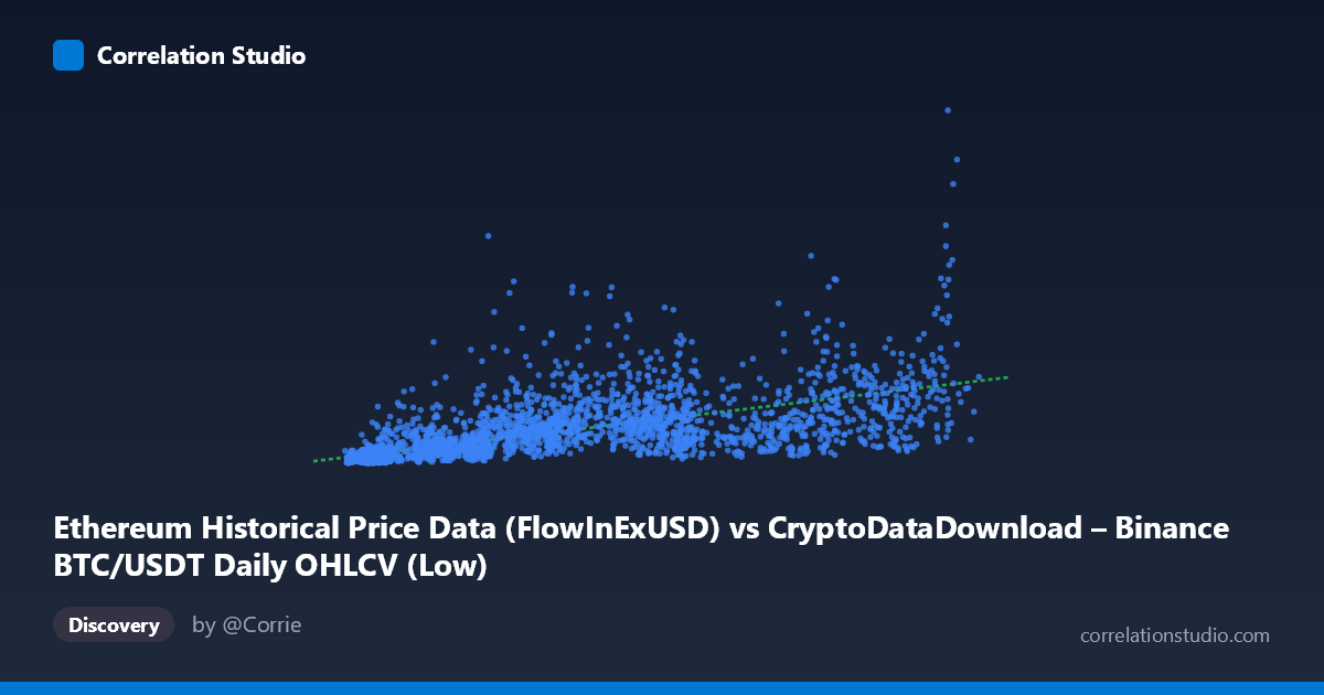
Ethereum Historical Price Data (FlowInExUSD) vs CryptoDataDownload – Binance BTC/USDT Daily OHLCV (Low)
- Pearson correlation (r)
- 0.648
- Spearman correlation
- 0.8115
- p-value
- 0
- Sample size (n)
- 3191
- 95% confidence interval
- 0.6274 to 0.6676
- Granger causality
- Y → X
- Granger optimal lag
- 10
AI analysis
Analysis of Ethereum/BTC Volume Flow Relationship
1. Overview of the Relationship
The scatterplot depicts a positive association between two flow/volume-related metrics tied to Ethereum and BTC/USDT trading activity. As X (Ethereum flow-in/exchange USD volume) increases, Y (associated Bitcoin low-price or volume metric) tends to rise as well, though with considerable scatter. The relationship is far from a tight linear band — many sample points show large vertical spread at similar X values (e.g., X≈6,000–10,000 spans Y from ~57M to ~588M), indicating that X alone is a weak-to-moderate predictor of Y's exact value, even though a general upward trend exists.
2. Strength, Direction, and Statistical Confidence
The Pearson correlation (r = 0.648) indicates a moderate positive linear relationship, with r² = 0.420 meaning only 42% of the variance in Y is explained by X — the majority (58%) is driven by other factors or noise. The 95% CI [0.627, 0.668] is tight given the large sample (n=3,191), and the p-value ≈ 0 confirms this correlation is highly statistically significant and not due to chance. However, statistical significance here reflects sample size more than practical predictive strength — r² of 0.42 leaves substantial unexplained variance for any real-world forecasting use.
The Granger causality results add an important temporal dimension: Y Granger-causes X (not the reverse), with the Y→X test significant (F=2.67, p=0.003) at a 10-period lag, while X→Y is not significant (p=0.140). This suggests that past values of the Bitcoin-related metric (Y) have predictive power over future Ethereum flow values (X) — the opposite direction from what the axis labels might naively suggest. This is a meaningful finding: correlation alone does not establish which variable "drives" the other, and here the temporal evidence points to Y leading X.
3. Patterns, Clusters, and Non-Linearity
Several notable features emerge: - Heteroscedasticity: Variance in Y increases substantially as X grows, forming a widening "fan" or cone shape — typical of financial/volume data with multiplicative rather than additive noise. - Low-X cluster with high-Y outliers: Several points with X < 10,000 show unexpectedly high Y values (e.g., X=9,900→Y=588M; X=6,430→Y=103M vs X=6,278→Y=144M), suggesting occasional volume spikes decoupled from the typical X-Y relationship. - Non-linearity flagged: The note that Spearman ρ exceeds Pearson r is a strong signal that a monotonic but curved relationship (log or power-law) fits better than a straight line. This is common in financial volume/price data, which often follows log-normal distributions. - The linear fit (y = 12,443.6x + 95.97M) likely underestimates Y at high X and overestimates at low X due to this curvature.
4. Confounding Factors and Caveats
- Shared market dynamics: Both BTC and ETH trade on correlated crypto markets; broader bull/bear cycles, macro liquidity, and exchange-wide volume surges likely drive both variables simultaneously (confounding via a common latent factor — overall market activity/sentiment). - Autocorrelation in time series: Both variables are time series with trends and volatility clustering; naive Pearson/Granger tests on non-stationary data can produce spurious correlations/causality. Differencing or detrending should be applied before drawing causal conclusions. - Cross-asset mismatch: The X and Y columns come from different underlying datasets (Ethereum flow-in vs. BTC/USDT low price), so the relationship may partly reflect exchange-level liquidity co-movement rather than a direct economic link between ETH and BTC. - Long time span (2017–2026): Structural market changes (regulation, halvings, DeFi growth) mean the relationship is unlikely to be stable across the whole period.
5. Recommendations for Further Investigation
- Re-fit using log-transformed variables (log-log or semi-log regression) given the fan-shaped variance and Spearman Pearson signal; this likely improves R² substantially. - Test stationarity (ADF/KPSS) before trusting the Granger causality result; consider re-running Granger tests on differenced/log-returns series to rule out spurious causality from shared trends. - Segment by market regime (bull vs. bear, or year-by-year) to see if the r=0.65 relationship holds consistently or is driven by specific high-volatility periods. - Investigate the low-X/high-Y outliers as potential distinct events (e.g., flash crashes, exchange outages, or specific news-driven volume spikes) that may warrant separate modeling. - Given Y leads X per Granger results, consider building an ARIMAX or VAR model using lagged Y to forecast X, rather than assuming a contemporaneous linear relationship.
X dataset: CryptoDataDownload – Binance BTC/USDT Daily OHLCV
Y dataset: Ethereum Historical Price Data
Part of experiment: Bitcoin - CryptoDataDownload – Binance BTC/USDT Daily OHLCV vs Ethereum Historical Price Data