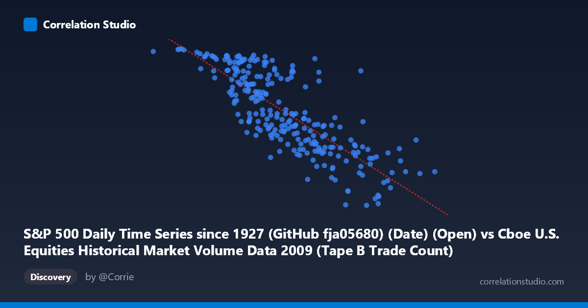
S&P 500 Daily Time Series since 1927 (GitHub fja05680) (Date) (Open) vs Cboe U.S. Equities Historical Market Volume Data 2009 (Tape B Trade Count)
- Pearson correlation (r)
- -0.8051
- Spearman correlation
- -0.8187
- p-value
- 0
- Sample size (n)
- 252
- 95% confidence interval
- -0.8447 to -0.7569
- Granger causality
- Bidirectional
- Granger optimal lag
- 10
AI analysis
Analysis: S&P 500 Opening Price vs. Cboe Tape B Trade Count (2009)
Relationship Overview The scatterplot reveals a clear negative relationship between the S&P 500 daily opening price and the Cboe Tape B Trade Count throughout 2009. As the S&P 500 opened at lower price levels (roughly 81,703 to ~400,000 on the x-axis, which likely represents a date-encoded or scaled value), trade counts tended to be higher, and as prices rose, trading activity declined. The linear regression equation y = −0.000744509x + 1,246.2 captures this inverse trend, showing that for every unit increase in the opening price index, the Tape B trade count decreases by approximately 0.000745 units. This pattern is visually consistent across the sample points, where lower x-values cluster around higher y-values (1,050–1,128) and higher x-values correspond to lower y-values (679–800).
Correlation Strength and Statistical Significance The correlation coefficient of r = −0.8051 indicates a strong negative linear association, and the R² of 0.6483 means that approximately 64.8% of the variance in Tape B trade counts is explained by the S&P 500 opening price — a substantial explanatory share, though roughly 35% of variance remains attributable to other factors. The 95% confidence interval of [−0.8447, −0.7569] is relatively narrow, reflecting high precision in this estimate given the large population (N = 3,232) and sample size (n = 252). The p-value of essentially zero confirms this relationship is highly statistically significant and almost certainly not due to chance. The Granger causality analysis adds important nuance: both directions show statistically significant results (X→Y: F = 2.23, p = 0.017; Y→X: F = 2.24, p = 0.017) at an optimal lag of 10 periods, indicating bidirectional temporal predictability. Neither variable cleanly "leads" the other — past S&P 500 prices help predict future trade counts, and past trade counts help predict future prices, suggesting a mutually reinforcing feedback dynamic rather than a simple one-way causal chain.
Notable Patterns, Clusters, and Outliers Several features stand out in the sample data. There is a visible cluster of high trade counts (1,080–1,128) associated with low x-values, notably the points near x ≈ 81,703 (y = 1,121), x ≈ 156,192 (y = 1,125), and x ≈ 208,484 (y = 1,108), which likely correspond to early 2009 market conditions during the financial crisis trough, when panic-driven trading volume surged. Conversely, the lowest trade counts (y ≈ 679–730) appear at x-values exceeding 600,000, consistent with mid-to-late 2009 recovery when the market stabilized and speculative urgency subsided. The point at x ≈ 766,764, y ≈ 775.87 appears as a potential high-leverage outlier at the far right of the distribution. There is also modest heteroscedasticity: scatter around the regression line appears wider in the mid-range of x, suggesting the linear model fits less precisely during transitional market periods.
Confounding Factors and Interpretive Caveats Several important caveats apply. First, the x-axis is described as an "Open" column from a date-indexed dataset, raising the possibility that x encodes a date or record index rather than a pure price level — if so, the correlation partly reflects the temporal arc of 2009 (crisis → recovery) rather than a direct price-volume mechanism. Second, macroeconomic confounders such as VIX volatility levels, Federal Reserve interventions, earnings seasons, and broad deleveraging dynamics in early 2009 could independently drive both lower prices and higher trade counts, inflating the apparent correlation. Third, Tape B specifically covers NYSE American (AMEX) and regional exchange activity, which may not perfectly represent aggregate market behavior. Fourth, while bidirectional Granger causality is detected, Granger causality measures predictive precedence, not true causal mechanism — the feedback loop observed may both be responses to a common latent driver (e.g., market stress).
Actionable Insights and Further Investigation Practitioners monitoring equity market microstructure should consider trade count as a coincident or slightly leading indicator of price stress, given the bidirectional Granger relationship at a 10-day lag. For risk management, spikes in Tape B trade counts during low-price environments may serve as an early warning signal worth incorporating into volatility models. Further investigation should include: (1) decomposing the temporal vs. price effect by regressing on both the date and opening price simultaneously; (2) extending the analysis to other Tape designations (Tape A for NYSE, Tape C for Nasdaq) to assess whether this pattern is exchange-specific; (3) incorporating VIX or realized volatility as a control variable to isolate the independent contribution of price level; and (4) testing whether the 10-period Granger lag corresponds to a meaningful trading calendar cycle (e.g., two weeks), which could inform algorithmic trading or rebalancing strategies.
X dataset: Cboe U.S. Equities Historical Market Volume Data 2009
Y dataset: S&P 500 Daily Time Series since 1927 (GitHub fja05680) (Date)
Part of experiment: Daily - Cboe U.S. Equities Historical Market Volume Data 2009 vs S&P 500 Daily Time Series since 1927 (GitHub fja05680) (Date)