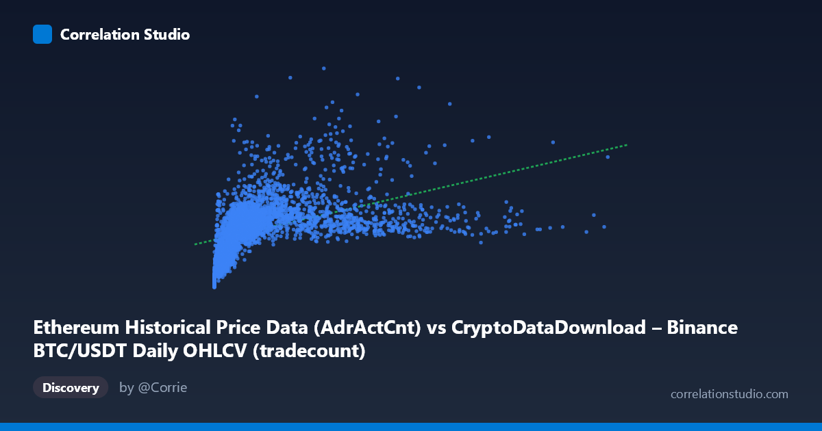
Ethereum Historical Price Data (AdrActCnt) vs CryptoDataDownload – Binance BTC/USDT Daily OHLCV (tradecount)
- Pearson correlation (r)
- 0.4623
- Spearman correlation
- 0.7086
- p-value
- 0
- Sample size (n)
- 3191
- 95% confidence interval
- 0.4346 to 0.4892
- Granger causality
- None
- Granger optimal lag
- 10
AI analysis
Analysis: BTC/USDT Metrics Relationship
1. What the Visualization Reveals
The scatterplot shows a moderate positive relationship between the X variable (mislabeled as "AdrActCnt" but contextually appears to be a BTC/USDT price or volume metric) and Y (tradecount). Data points cluster heavily in the lower-left region (X < 2,000,000, Y between 300,000–700,000), with a long right tail extending to X ≈ 15.36 million. This heavy-tailed distribution — where X's standard deviation (2.24M) exceeds its mean (1.97M) — indicates strong right-skew, meaning a small number of high-X observations are exerting outsized influence on the fitted line.
2. Strength, Direction, and Uncertainty
The Pearson correlation (r = 0.4623) indicates a moderate positive relationship, but r² = 0.2137 reveals that only about 21% of the variance in Y is explained by X — leaving nearly 80% attributable to other factors or noise. The 95% CI [0.434, 0.489] is reasonably tight given the large sample (n=3,191), and the p-value ≈ 0 confirms this correlation is highly unlikely to be due to chance. However, statistical significance here reflects sample size more than practical strength — a moderate r with a very large n almost always yields p≈0.
Critically, the Granger causality tests show no significant predictive direction in either direction (X→Y: p=0.50; Y→X: p=0.78). This means that past values of one series do not help forecast the other beyond what the series' own history provides, even at an optimal lag of 10 periods. Practically: despite being correlated contemporaneously, neither variable serves as a reliable leading indicator for the other in a time-series forecasting sense. The relationship may be driven by a shared external factor (e.g., overall market activity/volatility) rather than one variable causing changes in the other.
3. Notable Patterns and Outliers
Several features stand out: - Dense low-X cluster: The majority of points sit below X=2M, with Y ranging widely (150K–950K), suggesting high Y-variance even when X is low — a sign of a weak or non-linear relationship in this region. - Sparse high-X outliers: Points like (15.36M, ...) — implied by the range but not in the sample — and (8.27M, 976K), (8.70M, 573K), (6.03M, 538K) sit far from the bulk of data, potentially exerting high leverage on the regression slope. - Non-monotonic behavior at extremes: Some high-X points (e.g., 8.7M → Y=573K) show lower Y than mid-range X points (e.g., 4.19M → Y=999K), suggesting the relationship isn't strictly linear and may plateau or even reverse at high X. - Low-X, high-Y point: (152,364 → 614,264) and (259,212 → 466,227) show Y can be substantial even at very low X, reinforcing scatter/heteroskedasticity in the lower range.
4. Confounding Factors and Caveats
Several caveats limit interpretation: - Skewed X distribution: With mean/stdev ratio near 1, a log-transform of X is likely necessary — the note that Spearman ρ exceeds Pearson r supports this, indicating the true relationship may be monotonic but non-linear (e.g., logarithmic or power-law). - Metadata mismatch: The column labels are confusing — X is labeled "Ethereum...AdrActCnt" but described as BTC/USDT OHLCV data, while Y is labeled "tradecount" but attributed to an Ethereum dataset. This suggests possible data pipeline or labeling errors that should be resolved before drawing conclusions about what is actually being correlated (e.g., is this BTC price vs. ETH active addresses, or BTC trade count vs. something else?). - Time-varying market regimes: Crypto markets (2017–2026) experienced multiple bull/bear cycles; pooling all data ignores regime shifts (e.g., 2017 ICO boom, 2021 bull run, 2022 crash) that could create spurious aggregate correlation. - Autocorrelation: Both variables are likely non-stationary time series (trending, volatile), which can inflate Pearson correlation even absent a true causal link — Granger test results (showing no lead-lag relationship) support treating the raw correlation cautiously.
5. Actionable Insights
1. Clarify data provenance: Resolve the column/dataset labeling discrepancy before further analysis — verify what X and Y actually represent. 2. Re-fit with transformation: Given the skew and Spearman Pearson signal, test log-log or log-linear regression models; this will likely improve fit and better reflect the true functional form. 3. Segment by time regime: Break the 2017–2026 span into bull/bear/sideways periods and re-run correlation/Granger tests per regime to check for structural stability. 4. Check for a common driver: Since neither variable Granger-causes the other, investigate a third variable (e.g., overall market cap, volatility index, or macro liquidity conditions) that may jointly drive both. 5. Outlier robustness check: Re-run regression with high-leverage points (X 5M) removed or winsorized to see if r² and slope estimates are sensitive to these few extreme observations.
X dataset: CryptoDataDownload – Binance BTC/USDT Daily OHLCV
Y dataset: Ethereum Historical Price Data
Part of experiment: Bitcoin - CryptoDataDownload – Binance BTC/USDT Daily OHLCV vs Ethereum Historical Price Data