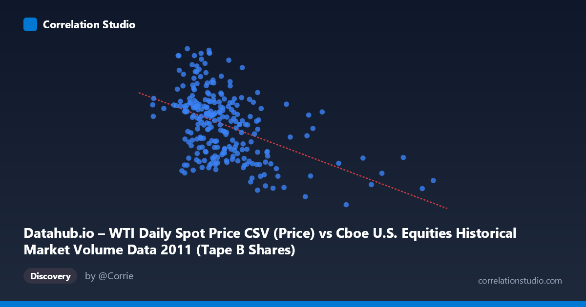
Datahub.io – WTI Daily Spot Price CSV (Price) vs Cboe U.S. Equities Historical Market Volume Data 2011 (Tape B Shares)
- Pearson correlation (r)
- -0.4664
- Spearman correlation
- -0.4474
- p-value
- 0
- Sample size (n)
- 252
- 95% confidence interval
- -0.5579 to -0.3638
- Granger causality
- None
- Granger optimal lag
- 1
AI analysis
Analysis: WTI Oil Price vs. Cboe Tape B Share Volume (2011)
Relationship Overview The scatterplot reveals a moderate negative relationship between U.S. equity market volume (specifically Tape B shares) and WTI crude oil spot prices across 252 trading days in 2011. As oil prices rose, Tape B share volumes on U.S. equity exchanges tended to decline, and vice versa. The linear regression equation (y = -1.14472E-07x + 106.116) captures this downward slope, though the scatter around the regression line is substantial, indicating that oil price alone is far from a complete explanation for daily equity trading volume behavior.
Correlation Strength and Statistical Significance The Pearson correlation of r = -0.4664 reflects a moderate negative association — directionally meaningful but not deterministic. More importantly, the coefficient of determination r² = 0.2176 indicates that only about 21.8% of the variance in Tape B share volume is explained by WTI prices, leaving roughly 78% attributable to other factors. The 95% confidence interval of [-0.5579, -0.3638] is entirely negative and does not cross zero, lending strong structural confidence to the direction of the relationship. The p-value of 5.107E-15 confirms the correlation is highly statistically significant given the population of N = 3,780, effectively ruling out chance as an explanation. However, Granger causality tests find no significant predictive directionality in either direction — neither X→Y (F = 0.0298, p = 0.8631) nor Y→X (F = 2.8605, p = 0.0920) clears the conventional 0.05 threshold. This critically means that while the two variables are correlated contemporaneously, neither reliably predicts the other's next-period movement, cautioning against any trading or forecasting strategy built on this relationship alone.
Notable Patterns and Outliers The sample points reveal considerable dispersion across the full range of oil prices (~$75–$113/barrel) and volume values. Several notable clusters and outliers are visible: a handful of high-volume observations (above ~108–113 Tape B shares) appear at both low and moderate oil prices, suggesting sporadic volume spikes unrelated to price level. At the higher end of oil prices (above ~$150–175M in X-axis units), volume observations seem to converge toward middling values rather than extreme lows, hinting at possible non-linearity or a floor effect in trading volume. Points like (62M, 111.68) and (101.9M, 110.60) represent high-volume outliers relative to the regression trend and may correspond to specific market events such as volatility spikes or macro announcements.
Confounding Factors and Caveats Several important caveats apply. 2011 was an unusually turbulent year — featuring the Arab Spring, Eurozone debt crisis escalation, the U.S. debt ceiling standoff, and S&P's downgrade of U.S. sovereign debt — all of which independently drove both oil price volatility and equity trading volume. These shared macroeconomic drivers could create spurious correlation: both variables responding to the same external shocks rather than influencing each other directly. Additionally, Tape B specifically covers NYSE American-listed securities, which skews toward smaller-cap stocks and may not generalize to broader market behavior. The lack of Granger causality also reinforces that this is likely a coincident relationship driven by common factors rather than a structural link.
Actionable Insights and Further Investigation Given these findings, analysts should avoid using oil prices as a direct predictor of Tape B equity volume in short-term models, given the failed Granger causality. More productive next steps would include: (1) introducing macro control variables such as VIX (volatility index), S&P 500 returns, or economic surprise indices to test whether the oil-volume correlation survives conditioning; (2) segmenting the analysis by market regime (e.g., pre- and post-August 2011 debt ceiling crisis) to identify whether the correlation is stable or driven by specific episodes; (3) testing non-linear models (e.g., polynomial or piecewise regression), as the scatter suggests the relationship may not be uniformly linear across the full oil price range; and (4) extending the time horizon beyond 2011 to assess whether this negative correlation is a structural feature of U.S. equity markets or an artifact of that year's specific macro environment.
X dataset: Cboe U.S. Equities Historical Market Volume Data 2011
Y dataset: Datahub.io – WTI Daily Spot Price CSV
Part of experiment: Daily - Cboe U.S. Equities Historical Market Volume Data 2011 vs Datahub.io – WTI Daily Spot Price CSV