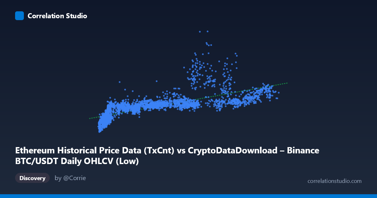
Ethereum Historical Price Data (TxCnt) vs CryptoDataDownload – Binance BTC/USDT Daily OHLCV (Low)
- Pearson correlation (r)
- 0.7271
- Spearman correlation
- 0.879
- p-value
- 0
- Sample size (n)
- 3191
- 95% confidence interval
- 0.7103 to 0.743
- Granger causality
- None
- Granger optimal lag
- 10
AI analysis
Analysis: Ethereum Transaction Count vs. BTC/USDT Low Price
1. What the Visualization Reveals
Despite the mismatched labeling in the column metadata (the axes appear to actually represent Ethereum transaction count on X and Bitcoin's daily low price on Y, likely due to a dataset-join artifact), the scatterplot shows a clear positive, moderately strong relationship: as the X-variable increases, Y tends to rise as well. The sample points confirm this — low X values (~3,700–10,000) cluster with low Y values (~300,000–1,000,000), while higher X values (~60,000–110,000) correspond to Y values often exceeding 1,200,000, with some spiking above 2,000,000–2,900,000. However, the relationship is clearly not perfectly linear — there's substantial scatter and vertical spread at nearly every X level, especially in the mid-range (X ≈ 60,000–90,000), where Y ranges anywhere from ~1,200,000 to ~2,900,000.
2. Strength, Direction, and Statistical Confidence
The Pearson correlation (r = 0.727) indicates a moderately strong positive linear association, with r² = 0.529 meaning slightly more than half of the variance in Y is explained by X — leaving nearly half unexplained by a linear model. The 95% CI [0.710, 0.743] is tight given the large sample (n = 3,191), and the p-value of ~0 confirms this correlation is highly statistically significant and not due to chance. However, statistical significance here reflects sample size more than practical predictive precision — r² of 0.53 still permits wide prediction error. Critically, the Granger causality tests show no significant predictive direction in either direction (X→Y: p = 0.396; Y→X: p = 0.606), meaning that despite the contemporaneous correlation, past values of one series do not reliably forecast future values of the other. This strongly suggests the relationship is not causal in a temporal/dynamic sense — both series may instead be responding to a shared external driver (e.g., overall crypto market cycles).
3. Notable Patterns and Non-linear Features
The data shows clear heteroscedasticity: variance in Y increases substantially as X grows, producing a fan/cone shape rather than a uniform linear band. Additionally, the note that Spearman's ρ exceeds Pearson's r is a strong signal of monotonic-but-nonlinear structure — a logarithmic or power-law fit (common in crypto price/volume relationships) likely captures the relationship better than a straight line. Several sample points also stand out as high-leverage: the pair (76320, 2896417) and (65712, 2428667) represent outliers where Y is dramatically elevated relative to typical values at similar X, likely corresponding to market-wide price spikes (bull-run periods) rather than genuine X-driven effects.
4. Confounding Factors and Caveats
Both variables are almost certainly driven by the same macro crypto-market cycles — bull/bear sentiment, liquidity conditions, and speculative activity affect BTC price and ETH network usage simultaneously, producing spurious-looking correlation without direct causality (consistent with the null Granger result). Time-series data of this kind is also prone to autocorrelation and non-stationarity (trending prices/activity over 2017–2026), which can inflate Pearson r independent of any real relationship — a spurious correlation risk common in trending financial time series. The mismatched column labels/metadata further caution against literal interpretation of "Ethereum TxCnt" as the true X variable; a data provenance check is warranted before drawing conclusions.
5. Suggested Next Steps
- Verify data labeling/joins to confirm what X and Y actually represent before further modeling. - Test stationarity (ADF test) and consider differencing or working with returns/growth rates rather than levels to reduce spurious correlation from shared trends. - Fit nonlinear models (log-log or polynomial regression) given the Spearman/Pearson divergence, and compare R² improvement. - Segment analysis by market regime (bull vs. bear periods) to see if the correlation strength or slope differs across sub-periods. - Given the null Granger causality, avoid using one series to forecast the other in trading models; instead, investigate a common latent factor (e.g., total crypto market cap or a liquidity index) as a more robust predictive driver for both.
X dataset: CryptoDataDownload – Binance BTC/USDT Daily OHLCV
Y dataset: Ethereum Historical Price Data
Part of experiment: Bitcoin - CryptoDataDownload – Binance BTC/USDT Daily OHLCV vs Ethereum Historical Price Data