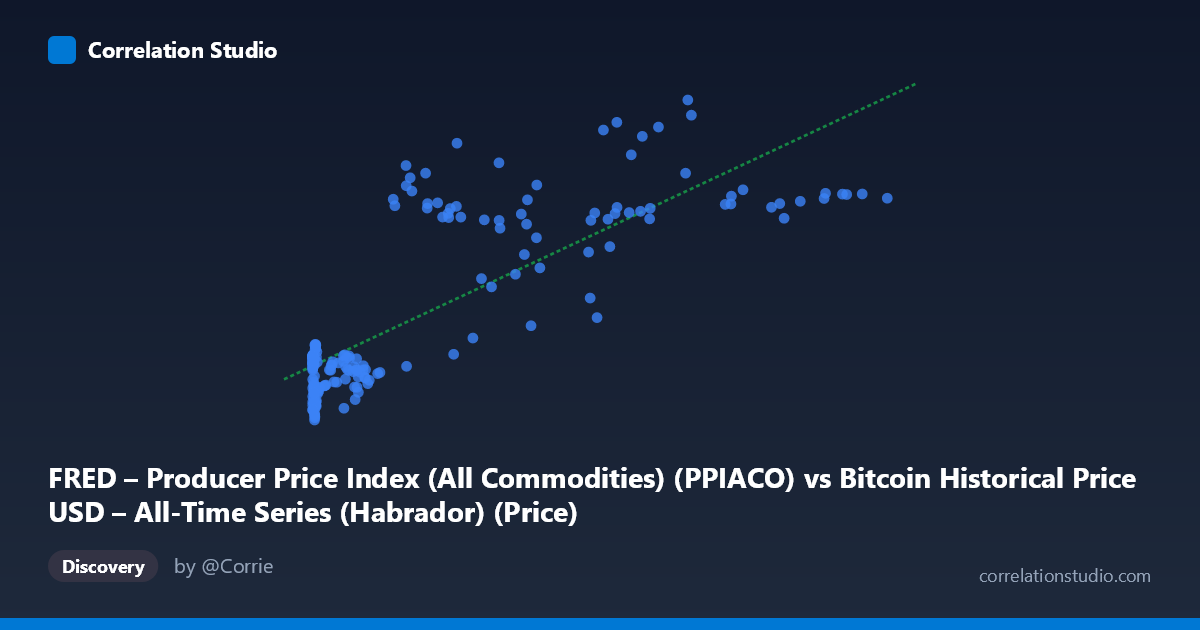
FRED – Producer Price Index (All Commodities) (PPIACO) vs Bitcoin Historical Price USD – All-Time Series (Habrador) (Price)
- Pearson correlation (r)
- 0.7956
- Spearman correlation
- 0.6469
- p-value
- 0
- Sample size (n)
- 189
- 95% confidence interval
- 0.7365 to 0.8427
- Granger causality
- None
- Granger optimal lag
- 2
AI analysis
Analysis: Bitcoin Price vs. Producer Price Index (PPIACO)
1. Relationship Overview
The scatterplot shows a strongly non-linear, log-like relationship between Bitcoin's USD price (X) and the Producer Price Index for All Commodities (Y). At low Bitcoin prices (under ~$1,000), PPI values cluster tightly in a relatively narrow band (roughly 181–210), showing little variation despite X spanning several orders of magnitude (0.06 to ~1,400). Once Bitcoin prices climb above $20,000–30,000, PPI values jump sharply upward into the 250–284 range. This creates a pattern that looks more like a step-function or saturating curve than a straight line, even though a linear fit is reported.
2. Strength, Direction, and Statistical Confidence
The reported r = 0.7956 (r² = 0.633) indicates a strong positive linear association, with the linear model explaining about 63% of the variance in PPI. The 95% CI [0.737, 0.843] is fairly tight and excludes zero, and the p-value of 0 confirms this correlation is highly unlikely to be due to chance in this sample. However, this is a classic case where correlation strength does not imply causal or mechanistic linkage: the Granger causality tests show no significant predictive direction in either direction (X→Y: p=0.224; Y→X: p=0.281). This means neither variable's past values help forecast the other's future values in a time-series sense — the strong r is likely driven by both series trending upward over the same calendar period (2010–2026) rather than one driving the other.
3. Notable Patterns and Outliers
Several features stand out: - Extreme X-axis compression: The vast majority of data points sit below X=2,000, while a handful of high-leverage points (X 60,000) anchor the upper-right of the trend line. This means the linear regression is disproportionately influenced by a small number of high-Bitcoin-price observations. - A visible outlier: (68074.00, 283.76) sits well above the general trend for that X range (other ~60-90K X values cluster around Y=253-262), suggesting either a data anomaly or a distinct economic event (e.g., a PPI spike unrelated to Bitcoin, such as a commodity inflation shock). - Plateau/step behavior: PPI seems to hold near ~190-205 for a long stretch of low Bitcoin prices (2010-2016 era), then transitions to a higher plateau (~250-260) for recent years — consistent with two macro regimes rather than continuous co-movement.
4. Confounding Factors and Caveats
The most important caveat: both series are dominated by a shared time trend, not necessarily a real economic relationship. Bitcoin price grew by ~6 orders of magnitude over this window while PPI rose due to general commodity inflation (including COVID-era supply shocks and monetary policy). Any two long-term upward-trending time series will show spurious high correlation. The non-Granger-causal result reinforces this — it's consistent with a "common trend" artifact rather than genuine interaction. Additionally, X's extreme right-skew (mean 20,533 vs. median likely far lower, stdev 29,894) means the Pearson r and linear R² are heavily influenced by a few large-X points; log-transforming X would likely produce a very different (probably weaker or differently-shaped) fit.
5. Actionable Insights
- Log-transform Bitcoin price before regression — given the multi-order-of-magnitude range, a log(X) vs. Y model would better capture the apparent saturating/logarithmic shape and likely improve fit interpretability. - Detrend both series (e.g., first-differencing or removing a common time trend) before testing correlation, to check whether the relationship survives after removing shared macro drift — this is critical since Granger tests already suggest no real predictive link. - Investigate the 68,074/283.76 outlier — verify it's not a data entry or alignment error between the two time series. - Treat this as a spurious/trend-driven correlation for any forecasting purpose; rely on the Granger results over the naive Pearson r when making claims about one variable driving the other.
X dataset: Bitcoin Historical Price USD – All-Time Series (Habrador)
Y dataset: FRED – Producer Price Index (All Commodities)
Part of experiment: Bitcoin - Bitcoin Historical Price USD – All-Time Series (Habrador) vs FRED – Producer Price Index (All Commodities)