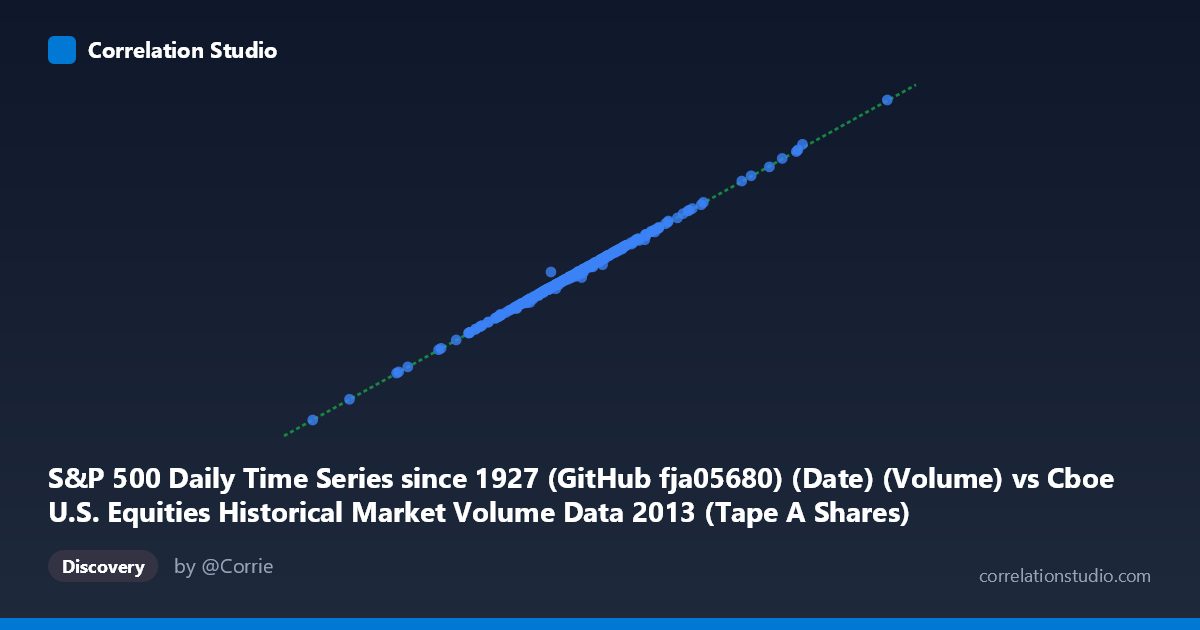
S&P 500 Daily Time Series since 1927 (GitHub fja05680) (Date) (Volume) vs Cboe U.S. Equities Historical Market Volume Data 2013 (Tape A Shares)
- Pearson correlation (r)
- 0.9993
- Spearman correlation
- 0.9982
- p-value
- 0
- Sample size (n)
- 252
- 95% confidence interval
- 0.9992 to 0.9995
- Granger causality
- Bidirectional
- Granger optimal lag
- 10
AI analysis
Analysis: S&P 500 Volume vs. Cboe Tape A Shares (2013)
Relationship Overview The scatterplot reveals a strikingly tight, positive linear relationship between S&P 500 daily trading volume (X-axis, sourced from GitHub fja05680) and Cboe U.S. Equities Tape A share volume (Y-axis) across 252 trading days in 2013. The data points cluster almost perfectly along the regression line y = 14.97x − 288,464, with virtually no visible scatter or deviation from linearity. This near-perfect alignment is visually immediate — the relationship looks less like a natural correlation and more like a near-deterministic mathematical identity, which itself is a critical observation worth scrutinizing carefully.
Correlation Strength and Statistical Significance The correlation is extraordinarily strong: r = 0.9993, with r² = 0.9987, meaning 99.87% of the variance in Tape A shares is explained by S&P 500 volume. The 95% confidence interval [0.9992, 0.9995] is vanishingly narrow, and the p-value is effectively zero across a paired sample of n = 252. These statistics collectively confirm that this is not a sampling artifact — the relationship is overwhelmingly robust. The Granger causality analysis reveals bidirectional causality at an optimal lag of 10 periods, with nearly symmetric F-statistics (X→Y: F = 2.56, p = 0.006; Y→X: F = 2.58, p = 0.006). This bidirectionality suggests neither series cleanly "leads" the other — both are likely driven by a shared underlying process rather than one causing the other in any meaningful economic sense.
Patterns, Clusters, and Outliers The sample points span X values from roughly 131M to 311M and Y values from ~1.97B to ~4.66B, with the bulk of observations clustering in the central range (X: 200M–265M, Y: 3.0B–4.0B). A handful of notable outliers are visible at the extremes — particularly the high-volume day near (310.8M, 4.66B) and the low-volume days around (131M, 1.97B) and (137M, 2.05B) — yet even these extreme points fall on or very near the regression line. There are no visible nonlinear features, heteroscedastic patterns, or distinct sub-clusters, reinforcing the interpretation that the relationship is uniformly linear across the entire volume range observed in 2013.
Confounding Factors and Caveats The most important caveat here is definitional overlap: both variables are measures of U.S. equity trading volume, just sourced from different datasets. S&P 500 volume aggregates constituent stock trades, while Tape A captures NYSE-listed share transactions — a substantial subset of the same universe. This means the correlation may reflect shared measurement infrastructure rather than any independent economic relationship. A correlation this close to 1.0 should trigger scrutiny about whether the two series are partially or fully derived from the same underlying data source, or whether one is arithmetically embedded within the other. The linear slope of ~14.97 (Tape A shares ≈ 15× S&P 500 volume units) likely reflects a unit-scaling difference rather than a behavioral relationship. The bidirectional Granger causality at lag 10 may also be a statistical artifact of this near-identity, rather than evidence of genuine predictive dynamics.
Actionable Insights and Further Investigation Before drawing any market-behavioral conclusions, the primary investigative priority should be verifying the independence of these two data series — specifically whether the S&P 500 volume figures (from Yahoo Finance via GitHub) and Cboe Tape A volumes are truly distinct measurements or overlapping aggregations of the same trades. If confirmed as independent, the relationship would be a genuinely powerful cross-source validation tool, useful for data quality checks or imputation when one series has missing values. Further analysis should disaggregate by market condition regimes (e.g., high-volatility vs. low-volatility days), test whether the relationship holds across other years (the 2013 sample is a single calendar year), and examine residuals microscopically — even tiny systematic deviations from linearity could reveal meaningful signal. Researchers should also explore whether the ~10-day lag in Granger causality aligns with known settlement cycles or reporting delays, which could offer a more mechanistic explanation for the temporal structure.
X dataset: Cboe U.S. Equities Historical Market Volume Data 2013
Y dataset: S&P 500 Daily Time Series since 1927 (GitHub fja05680) (Date)
Part of experiment: Daily - Cboe U.S. Equities Historical Market Volume Data 2013 vs S&P 500 Daily Time Series since 1927 (GitHub fja05680) (Date)